Impact of adopting improved Arabica varieties on the livelihood of organic coffee producers’ of Ethiopia: Continuous treatment approach

Abstract

The study evaluated the impact of adopting improved coffee Arabica on organic coffee producers’ households’ livelihoods by employing data obtained from 120 coffee producer households in the Gedeo zone. The generalised propensity-score matching methodology is used to analyse the data. The approach was used to match families with similar variables and varying levels of enhanced Arabica coffee adoption intensity. The technique proved efficient in elucidating non-linear causal links between adoption intensities, dosages, and outcome variables. The average dose-response or impact function was calculated by averaging consumer expenditure, household per capita income, and calorie intake per AE at various levels of adoption intensities. The result showed that initially, coffee production had a negative impact on kilocalories per adult equivalent (AE) but turned positive following an adoption dose that reached the optimum. The improved Arabica coffee varieties’ optimal adoption dose is 71.42%, and the equivalent annual household calorie consumption is 2,384.80 kilocalories per AE. However, the impact of coffee Arabica adoption on consumption expenditure was initially positive, but it turned negative after the adoption dose reached its optimum. The level of optimum adoption is 28.41, and the annual household consumption expenditure was 13704 Ethiopian Birr. Furthermore, at an optimum level of 83.66%, the intensity of adoption and income of coffee producers had a positive impact. In this context, policies that promote the efficiency of coffee production and minimize the barriers to farmer adoption provide the most optimal land allocation for improved technology and, in doing so, improve the lives of households.

Keywords:

• Impact
• Generalized Propensity Score
• Livelihood
• Southern Ethiopia

REVIEWING EDITOR:

• M. Luisa scudero-Gilete, Nutrition and Bromatology, Universidad de Sevilla, Sevilla, Spain

SUBJECTS:

• Environment & Economics
• Development Studies
• Rural Development
• Econometrics

Introduction

Ethiopia stands as Africa’s foremost coffee producer, holding the esteemed rank of the 5th largest producer of this coveted crop on a global scale (Moat et al., 2017). The nation’s annual coffee production reportedly lies within the range of 500,000 to 700,000 metric tons, with a national productivity average of seven quintals per hectare, as per the CSA (2018). Notably, Ethiopia’s coffee production not only plays a pivotal role in its economy but also contributes significantly to its export value, accounting for 34% of all export value in the 2017/18 period (GAIN, 2019). The country’s coffee export trend has shown upward momentum, escalating from 238,465.55 metric tons in 2017/18 to 225,667.67 metric tons in 2016/17, with an anticipated increase to 249 metric tons expected by 2020/21, solidifying its status as the leading African coffee exporter and the world’s tenth largest exporter (Tollera, 2020; USDA, 2020).

Given the paramount importance of this commodity, the government has particularly intensified its focus on the coffee sector, with it being the inaugural cash crop traded on the Ethiopia Commodity Exchange (ECX) since April 2008, an initiative aimed at fortifying the country’s coffee markets (Gelaw et al., 2016). It’s noteworthy to mention that prior to the establishment of ECX, coffee producers grappled with inadequate access to credit, market information, transportation, and other essential resources (Perfect Daily Grind, 2020). Indeed, despite substantial governmental efforts to enhance coffee marketing, a study by Amsalu (2015) highlights that farmers continue to face challenges in productivity and production. These hurdles disproportionately impact smallholder coffee producers, who cultivate 90% of the coffee on average on small-scale farms spanning 0.5–2 hectares (Solymosi and Techel, 2019), leading to diminished foreign exchange earnings for the country.

In light of these challenges, ensuring sustainable coffee productivity and market success in Ethiopia emerges as a paramount goal to bolster the livelihoods of coffee producers. Achieving this entails leveraging cost-effective, productivity-boosting agricultural technologies and facilitating improved access to product markets (Ayele et al., 2021), recognizing that increasing productivity through expanding the cultivated area, particularly in coffee-producing areas, is constrained by population pressure. Consequently, elevating productivity levels and streamlining product market access are pivotal mechanisms to alleviate these issues and enhance the livelihoods of farmers. Essentially, by enriching the economic capacity of coffee producers, it becomes viable to uplift societies in coffee-producing areas and meet their needs, despite coffee being categorized as a non-food crop.

There have been numerous studies conducted to assess the impacts of enhanced agricultural technologies on different aspects of livelihood and welfare. For instance, Kassie et al. (2011) conducted a study in Uganda to investigate the impact of technology adoption on poverty and production costs. Similarly, studies by Amare et al. (2012) and Irene et al. (2018) have examined the welfare and poverty reduction impacts of adopting improved agricultural technologies in Tanzania. In China, studies by Ma and Abdulai (2019), Gao et al. (2019), Tufaa et al. (2019), Hou et al. (2020), Huang et al. (2020), and Wu (2022) have focused on the impact of these technologies on farmer production and net income. In Africa, studies by Mignouna et al. (2011), Makate et al. (2017), and Houeninvo et al. (2019) have explored the impact on farm household income.

The majority of these studies have utilized the propensity score matching (PSM) technique. However, it is important to note that these studies have assumed the benefits to be constant and uniform across all families, regardless of the extent to which better Arabica coffee varietals are adopted. By considering adoption as a binary process, these studies have provided an average treatment impact assessment, assuming all adopter households to be at the same level of adoption. Consequently, PSM fails to capture the diverse impacts of adoption. It is critical to look at the distribution of impacts beyond the mean in order to gain a more realistic understanding of how adoption affects well-being and to gather evidence that either supports or refutes economic theories that imply heterogeneous responses (Djebbari & Smith, 2008).

Given that adoption impacts are expected to vary based on the level of adoption, it is reasonable to assume that not all adopters will benefit equally. However, only a few studies, such as those conducted by Kassie et al. (2014), have utilized the generalized propensity score (GPS) method to assess the impact of enhanced agricultural technologies on households’ food security in Tanzania. This study aims to contribute to the existing body of literature by utilizing the generalized propensity score (GPS) method to examine the impacts of improved Arabica coffee varieties on calorie intake per adult equivalent (AE), consumption expenditure, and income of farm households in the Gedeo administrative zone of southern Ethiopia.

The Gedeo zone is known for producing some of the highest-quality organic coffee in the world (World Vision, 2020). The Gedeo agricultural system stands out for its use of organic inputs throughout the production process (Abdu & Gedeo, 2013; Kippie, 2002; Kodama, 2007). Yirgacheffe and Sidama brand coffees are among the many certified organic agricultural products from the area (Abdu and Gedeo, 2013; Kodama, 2007; Negash, 2013). However, despite this, most smallholder organic coffee producers in the area live below the national standard food poverty line (Shumete, 2009), indicating widespread poverty and food insecurity. It is possible that smallholder farmers have not reaped significant benefits from their coffee production. The same holds true for the Kochore district, where poverty and food insecurity persist despite the reliance on internationally traded commodities. Poor productivity is cited as a leading cause of these issues in the area, with limited use of technologies such as improved coffee varieties contributing to inefficient performance (DANRB (District Agriculture and Natural Resource Bureau, 2021).

This study utilized GPS to assess the impacts of adopting improved Arabica coffee varieties on the livelihoods of coffee farmers. The researchers hypothesized that adoption impacts may vary depending on the degree of adoption, suggesting that not all adopters may benefit equally. Therefore, it is important to consider this heterogeneity when evaluating its impact to avoid producing inaccurate information. The study aims to answer the research question: Have improved Arabica coffee varieties impacted the calorie intake, consumption expenditure, and income of organic coffee grower households in the Gedeo Zone of southern Ethiopia, controlling for adoption differences?

Study area

The study was undertaken in the Gedeo Zone of southern Ethiopia. The zone is located 365 kilometres from the capital city, Addis Ababa. The total land area covered by the zone is 134,700 ha. Kochore district is among the districts of the Gedeo zone, situated 90 km from the regional capital of Hawassa and 375 km southeast of Addis Ababa (CSA, 2015). It has 26 rural kebeles and a municipality with three urban kebeles. The total population of the districts is 164,893, of which 81,804 are men and the other 83,086 are women. The district’s total area is 20119.54 hectares, of which 95% is cultivated. Of this, 15,732.18 hectares were covered by coffee plantations, and 3381.38 hectares were covered by other crops (CSA, 2015). The study district has a bimodal rainfall distribution that stretches from 1000–1200 mm and a mean annual temperature of 15.1 °C–20 °C (SNNPR, 2018). Rugged topography, a humid climate, and mixed farming are the dominant modes of production in the district. The district has organic, forest-based, garden coffee cultivation experience spanning centuries. The study area is ideal for producing high-quality Arabica coffee because of its natural climate, geography, and ecosystem (World Vision, 2020).

Methods

Sampling procedure and data collection methods

Of the 26 kebeles in the Kochore district, 18 kebeles¹ are prominently known for coffee production. From the 18 kebeles known for producing organic coffee, 6 kebeles were selected randomly. After securing a fresh list of household heads from the six kebeles, households were again stratified into adopter groups (who have adopted improved coffee varieties) and non-adopter groups (who have not adopted). The users of improved coffee varieties are the only ones included in this study. Finally, a sample of 120 adopters of improved coffee-producing households was randomly chosen. The survey was conducted during the period of February and March 2021, employing a one-on-one interview format. Skilled and experienced enumerators, well-versed in the local language, were responsible for carrying out the survey. They utilized a pre-tested, structured questionnaire to gather the necessary data.

Generalized propensity score (GPS) method

The best analytical approach most commonly used for impact evaluation by social science researchers is propensity score matching (PSM) if the treatment is binary and not randomized (Rosenbaum and Rubin 1983). The GPS method, on the other hand, is an appropriate tool for an empirical analysis of the dose-response function when the treatment (social interventions) variable is continuous in nature and value (Hirano and Imbens 2004). Furthermore, the literature suggests that the GPS method is the right tool for the evaluation of social sciences (Bia and Mattei, 2008; Kassie et al., 2014; Kluve et al., 2012; Li and Fraser, 2015; Liu and Florax, 2014; Zhai et al., 2010).

Currently, GPS has been widely used in different intervention evaluation literature. Random sample units from a large population and indexed by i = 1, …, N was assumed. For each unit i in t level of treatment, there is a potential set of outcomes {Yi(t)} tєT refers to the dose-response function (DRF). In the dummy treatment variable, T = {0, 1} difference in adoption level of improved coffee Arabica varieties T is in the interval [t₀, t₁], with t0 > 0 (Hirano and Imbens, 2004). The focus of the study captures only the average dose-response and marginal treatment functions of adopters of improved coffee producer households. As a rule, missing data problems are natural for impact evaluation research. Thus, identifying the curve of average potential outcomes is the main focus of interest (Kassie et al., 2014). In this study, µ(t) = E[Yi(t)] stands for the average potential livelihood outcomes function of the overall possible adoption levels of improved coffee varieties, and Yi(t) is a livelihood indicator including household income, household expenditure, and household consumption for a household affected by adoption.

The observable variables for each unit i are a covariate vector Xi, the level of the treatment received by the unit is Ti with Tiє(t₀, t₁), and the corresponding potential outcome level received by treatment is Yi = yi(Ti). The GPS application’s focus only considers households that adopt improved coffee varieties’ average dose-response and marginal treatment functions. Similar to the dummy matching approach, GPSM abides by weak unconfoundedness assumptions and balancing properties.

The assumption of weak unconfoundedness states implied the following observable characteristics X_i controlling, the treatment intensity of any difference remaining in T_i across units is not related to the potential outcomes of Y_i (t), Equation (1)(1) $$Y_i\left(t\right)\perp T_i/X_i\mathrm{ }\mathit{\text{for all}}\mathrm{ }t\in T\mathrm{ }$$(1) . (1) $$Y_i\left(t\right)\perp T_i/X_i\mathrm{ }\mathit{\text{for all}}\mathrm{ }t\in T\mathrm{ }$$(1)

The reason for referring to the weak unconfoundedness is that the mutual exclusiveness of all potential outcomes is that treatment with every potential outcome involves only pairwise conditional independence of treatment (Hirano & Imbens, 2004). The random variable treatment Ti is assumed to be conditionally independent from the random outcome variable Yi, measured at an arbitrarily chosen treatment level t. Therefore, under a weak unconfoundedness assumption, the average dose-response function estimation should be captured by considering the average potential outcomes and different treatment levels. This facilitates the process of isolating an adoption’s impact. To put it another way, GPS aids in the elimination of any potential biases brought on by variations in variables (Hirano and Imbens 2004.

As shown in Equation (2)(2) $$R_i=⊺(T_{i\mathrm{ }},X_i)$$(2) , the GPS balancing property is represented as r(t, x) = T/X(t/x), the conditional density of the treatment given the covariates. (2) $$R_i=⊺(T_{i\mathrm{ }},X_i)$$(2)

Within strata, the probability that T= t does not depend on the value of X, i.e. X┴1{T = t}|r(t, X) becomes a GPS property, as long as the same value of r(t, X) is obtained within strata, the possibility that T= t is independent of the X value. Hirano and Imbens (2004) focus on a mechanical inference of the GPS definition and do not necessitate unconfoundedness; given the GPS, the treatment assignment is unconfounded. According to Hirano and Imbens (2004), if a weakly unconfounded assignment to treatment is given covariate X, then given the GPS, it is also weakly unconfounded. As a result, GPS biases associated with differences in the observed covariates can be removed. If the assignment to treatment is weakly unconfounded by pretreatment variables X, Hirano and Imbens (2004) calculate β(t, r) = E [Yi(t)|r(t, Xi)] = E [Yi|Ti = t, Ri = r]; and (t) = E [(t, r) (t, Xi)]. Accepting the result, using the GPS bias associated with differences in covariates removed in two steps and the third step using a partial mean approach, the dose-response function estimate at a particular treatment level t.

First, calculate the GPS—the conditional treatment density given the covariates. Following the first step estimate, the outcome conditional expectation of two scalar variables function, Equation (3)(3) $$\beta \mathrm{ }\left(t,r\right)=E\left[Y/T=t,R=r\right]$$(3) specification shows the GPS R and the treatment level T. (3) $$\beta \mathrm{ }\left(t,r\right)=E\left[Y/T=t,R=r\right]$$(3)

In step three, the DRF at each treatment level should be estimated. Using Equation (4)(4) $$\mu \left(t\right)=E\left[\beta \left(t,r\left(t,X\right)\right)\right],t\forall T\mathrm{ }$$(4) , averaging the conditional expectation function over the GPS at that particular level of treatment has been implemented. (4) $$\mu \left(t\right)=E\left[\beta \left(t,r\left(t,X\right)\right)\right],t\forall T\mathrm{ }$$(4)

The R = r (T, X) estimation procedure does not allow for an average over the GPS; instead, it averages over the score estimated at the level of treatment of interest r(t, X). Hirano and Imbens (2004) as well confirm that there is no causal interpretation for the estimate of the regression function β(t, r); nevertheless, μ(x) refers to the DRF value for treatment value t compared to another treatment level t, which does have a causal interpretation.

Three main steps are followed for the practical application of GPS in estimating the adoption impacts of improved coffee varieties at different adoption intensities in the study areas (Hirano and Imbens, 2004). The first step is to evaluate the GPS as a conditional density of treatment given covariates using a flexible parametric approach. Given the covariates, the adoption of coffee varieties is assumed to be distributed normally. Thus, the treatment function parameters indicated in Equation (5)(5) $$T_i∕X_i\sim N[{\beta }_0+{\beta }_1{X}_i+{\delta }^2$$(5) are estimated based on maximum likelihood. (5) $$T_i∕X_i\sim N[{\beta }_0+{\beta }_1{X}_i+{\delta }^2$$(5)

It is noted that the GPS estimation is vital to balancing the covariates across the categories of treatment; once an adequate balance of covariates is attained, the GPS procedures used to estimate them are of secondary importance (Kluve et al., 2012). Before moving on to the next step of GPS estimation, its balancing property should be tested. Subsequent to the parameter estimation of the treatment function following Equation (5)(5) $$T_i∕X_i\sim N[{\beta }_0+{\beta }_1{X}_i+{\delta }^2$$(5) , Equation (6)(6) $${\overbrace{R}}_i\mathrm{ }\frac{1}{\sqrt{2\prod {\delta }^2}}\mathrm{ }\mathrm{\text{exp}}[-\frac{1}{2\overbrace{{\delta }^2}}\mathrm{ }[\mathrm{ }{T}_i‐\mathrm{ }{\overbrace{\beta }}_0‐\mathrm{ }{\overbrace{\beta }}_1{X}_i{)}^2]$$(6) could be used to estimate GPS. (6) $${\overbrace{R}}_i\mathrm{ }\frac{1}{\sqrt{2\prod {\delta }^2}}\mathrm{ }\mathrm{\text{exp}}[-\frac{1}{2\overbrace{{\delta }^2}}\mathrm{ }[\mathrm{ }{T}_i‐\mathrm{ }{\overbrace{\beta }}_0‐\mathrm{ }{\overbrace{\beta }}_1{X}_i{)}^2]$$(6)

Step two, the outcome conditional expectation. In this study, rural livelihood indicator(s) (Yi) is modelled using the polynomial approximation that involves the interactions of observed treatment (Ti) and GPS (Ȓi) estimated (Hirano and Imbens, 2004). For instance, if the quadratic approximation is followed, Equation (7)(7) $$\begin{array}{l}\beta \left(t,\hspace{0.17em}r\right)=g\left(\left[\frac{Y_i}{T_i},\hspace{0.17em}\stackrel{}{\stackrel{︷}{\mathit{\text{Ri}}}}\right]\right)\\ =\hspace{0.17em}{\alpha }_0+\hspace{0.17em}{\alpha }_1{T}_i+\hspace{0.17em}{\alpha }_2{T}_I^2+\hspace{0.17em}{\alpha }_3\stackrel{}{\stackrel{︷}{R}}i+\hspace{0.17em}{\alpha }_4{\stackrel{}{\stackrel{︷}{R}}}_i^2+\hspace{0.17em}{\alpha }_4{T}_i\stackrel{}{\stackrel{︷}{R}}i\end{array}$$(7) is in order. (7) $$\begin{array}{l}\beta \left(t,\hspace{0.17em}r\right)=g\left(\left[\frac{Y_i}{T_i},\hspace{0.17em}\stackrel{}{\stackrel{︷}{\mathit{\text{Ri}}}}\right]\right)\\ =\hspace{0.17em}{\alpha }_0+\hspace{0.17em}{\alpha }_1{T}_i+\hspace{0.17em}{\alpha }_2{T}_I^2+\hspace{0.17em}{\alpha }_3\stackrel{}{\stackrel{︷}{R}}i+\hspace{0.17em}{\alpha }_4{\stackrel{}{\stackrel{︷}{R}}}_i^2+\hspace{0.17em}{\alpha }_4{T}_i\stackrel{}{\stackrel{︷}{R}}i\end{array}$$(7)

Here, g represents a function of the outcome variable. Using regression models for continuous rural livelihood outcome variables, including household income, consumption expenditure, and calorie intake, is not unusual. Therefore, the parameters of the GPS result are obtained through OLS ${\widehat{\mathrm{R}}}_{\mathrm{i}}$. Note that the coefficient results obtained using Equation (7)(7) $$\begin{array}{l}\beta \left(t,\hspace{0.17em}r\right)=g\left(\left[\frac{Y_i}{T_i},\hspace{0.17em}\stackrel{}{\stackrel{︷}{\mathit{\text{Ri}}}}\right]\right)\\ =\hspace{0.17em}{\alpha }_0+\hspace{0.17em}{\alpha }_1{T}_i+\hspace{0.17em}{\alpha }_2{T}_I^2+\hspace{0.17em}{\alpha }_3\stackrel{}{\stackrel{︷}{R}}i+\hspace{0.17em}{\alpha }_4{\stackrel{}{\stackrel{︷}{R}}}_i^2+\hspace{0.17em}{\alpha }_4{T}_i\stackrel{}{\stackrel{︷}{R}}i\end{array}$$(7) are vital to test the overall significance of the variables; it refers to checking the existence of bias among the covariates (Hirano and Imbens, 2004).

Hirano and Imbens (2004) further outlined that in empirical analysis using the estimated parameters ($\widehat{\mathrm{\alpha }}$) in step two, the average outcome treatment (t) level and an entire dose-response function were calculated. In other words, the average dose-response function for each treatment level t estimates the conditional expectation average ß(t, r) using Equation (8)(8) $$\begin{array}{l}\mu \left(t\right)=E\left[\stackrel{�}{Y}\left(t\right)=\frac{1}{N}{\displaystyle \sum }_{i=1}^N{g}^{-1}\right[{\stackrel{�}{\alpha }}_0+\hspace{0.17em}{\stackrel{�}{\alpha }}_{1}t+\hspace{0.17em}{\stackrel{�}{\alpha }}_2{t}^2+\hspace{0.17em}{\stackrel{�}{\alpha }}_3\stackrel{�}{r}\left(t,\hspace{0.17em}{X}_i\right)\\ +\hspace{0.17em}{\stackrel{�}{\alpha }}_3\stackrel{�}{r}\left(t,\hspace{0.17em}{X}_i\right)2+\hspace{0.17em}{\stackrel{�}{\alpha }}_{5}t\stackrel{�}{r}\left(t,\hspace{0.17em}{X}_i\right)]\end{array}$$(8) . (8) $$\begin{array}{l}\mu \left(t\right)=E\left[\stackrel{�}{Y}\left(t\right)=\frac{1}{N}{\displaystyle \sum }_{i=1}^N{g}^{-1}\right[{\stackrel{�}{\alpha }}_0+\hspace{0.17em}{\stackrel{�}{\alpha }}_{1}t+\hspace{0.17em}{\stackrel{�}{\alpha }}_2{t}^2+\hspace{0.17em}{\stackrel{�}{\alpha }}_3\stackrel{�}{r}\left(t,\hspace{0.17em}{X}_i\right)\\ +\hspace{0.17em}{\stackrel{�}{\alpha }}_3\stackrel{�}{r}\left(t,\hspace{0.17em}{X}_i\right)2+\hspace{0.17em}{\stackrel{�}{\alpha }}_{5}t\stackrel{�}{r}\left(t,\hspace{0.17em}{X}_i\right)]\end{array}$$(8)

$\widehat{\alpha }$ the vector of estimated parameters in step two $\widehat{r}\left(t,{{\displaystyle X}}_i\right)$ is the value predicted r(t, X_i) treatment at level t. The dose-response function is entirely attained by calculating the average potential outcome of the treatment for each level. Besides Equation (8)(8) $$\begin{array}{l}\mu \left(t\right)=E\left[\stackrel{�}{Y}\left(t\right)=\frac{1}{N}{\displaystyle \sum }_{i=1}^N{g}^{-1}\right[{\stackrel{�}{\alpha }}_0+\hspace{0.17em}{\stackrel{�}{\alpha }}_{1}t+\hspace{0.17em}{\stackrel{�}{\alpha }}_2{t}^2+\hspace{0.17em}{\stackrel{�}{\alpha }}_3\stackrel{�}{r}\left(t,\hspace{0.17em}{X}_i\right)\\ +\hspace{0.17em}{\stackrel{�}{\alpha }}_3\stackrel{�}{r}\left(t,\hspace{0.17em}{X}_i\right)2+\hspace{0.17em}{\stackrel{�}{\alpha }}_{5}t\stackrel{�}{r}\left(t,\hspace{0.17em}{X}_i\right)]\end{array}$$(8) , several other specifications should be implemented to ensure adequately flexible functional forms (Kluve et al., 2007). The GPS analysis estimates have been indicated graphically. The functions of average dose-response plots and marginal treatment effects, defined as the corresponding dose-response function derivatives, should be shown graphically.

The average dose-response function depicts the intensity and nature of the causal relationship between adoption and the outcome variables (consumption expenditure, household per capita income, and caloric intake per AE). The "doseresponse2" STATA 16 software command was used for data analysis (Guardabascio and Ventura, 2014; Kassie et al., 2014).

Adoption intensity of improved coffee Arabica varieties is a continuous variable measured as the percentage of the total land covered by improved coffee Arabica varieties. Regarding the measurement of the outcome variables, annual income refers to household income earned from off-farm and farm activities, measured in Ethiopian Birr (ETB).² Likewise, consumption expenditure includes spending on food and non-food items in ETB. Furthermore, calorie intake per adult equivalent is measured by looking at two weeks’ period of data on the food available for consumption in sample households. This involves converting purchase and stock data into kilocalories and subsequently dividing the resulting figures by the total adult equivalents in each household.

Variable definitions, measurement and working hypothesis Used in GPSM model are presented in Table 1.

Table 1. Variable definitions, measurement and working hypothesis.

Variable	Variable description and measurement	Hypothesis
Treatment variables
Intensity of adoption of improved coffee Arabica varieties	Continuous; Percentage of total land area covered by improved coffee Arabica varieties
Outcome variables
Household per capita income	Continuous; Ethiopian birr
Consumption expenditure per adult equivalent	Continuous; Ethiopian birr
Calorie intake per adult equivalent	Continuous; kilocalories per adult equivalent
Explanatory variables
Age of household head	Continuous; years	+
Years of schooling	Continuous; education level attained	+
Family size	Continuous; number of family members	+
Livestock holding (TLU)	Continuous; Tropical livestock unit	+
Distance to market	Continuous; hours	–
Distance main road	Continuous; hours	–
Distance to get improve seed	Continuous; hours	–
Age square	Continuous; years square	–
Age cube	Continuous; years cube	–
TLU square	Continuous; Tropical livestock unit square	–
TLU cube	Continuous; Tropical livestock unit cube	–
Education level square	Continuous; education level attained square	+
Education level cube	Continuous; education level attained cube	+
Family size square	Continuous; number of family members square	+
Family size cube	Continuous; number of family members cube	+
Distance main road square	Continuous; hours square	–
Distance main road cube	Continuous; hours cube	–
Distance to get improve seed square	Continuous; hours square	–
Distance to get improve seed cube	Continuous; hours cube	–

Results and discussion

Descriptive results

Adoption intensity and socio-economic characteristics of sample households

Table 2 shows the farm households grouped into three based on the adoption intensity score difference (i.e., 30%, 70%) following Kluve et al. (2007).

Table 2. Sample households’ distribution by adoption intensity score group.

Variable	Treatment interval with GPS estimate	No.	%
Group 1	≤ 0.498753	35	29
Group 2	0.498753 to 0.731707	50	42
Group 3	≥ 0.731707	35	29

Table 3 shows that out of 120 randomly selected farm households, 90% are male-headed, while the rest, 10%, are female-headed farm households. The average age of the sample households was 46.64 years. Among the 120 adopters of improved varieties, 29.2% were categorised as low adopters, 41.6% were medium adopters, and the rest, 29.2%, were high adopters. Household head participation in off-farming activities comprised 23.33% of participants, and the remaining 76.67% were non-participants. The chi-square test at the 5% level of significance indicated that there is a difference in off-farm economic activity engagement among households with low, medium, and high adoption levels. Of the 120 sample respondents, 33.33% have access to credit, whereas 66.67% have no access to credit for most of the sample.

Table 3. Socio-economic characteristics of sample households by the intensity of adoption.

Variables	Description	Low		Medium		High		Total
		(N = 35)		(N = 50)		(N = 35)		(N = 120)
		No.	%	No.	%	No.	%	No.	%
Sex of the head (1 = male)	Male	33	94.29	44	88	31	88.57	108	90	1.016NS
	Female	2	5.71	6	12	4	11.43	12	10
Off-farm income participation (1 = yes)	Yes	13	37.14	7	14	8	23.53	28	23.33	6.170**
	No	22	62.86	43	86	27	79.41	92	76.67
Credit use (1 = yes)	Yes	12	34.29	17	34	11	31.43	40	33.33	0.081NS
	No	23	65.71	33	66	24	68.57	80	66.67

Note: **means significant at the 5 percent probability level.

As indicated in Table 4, there is no significant difference between the three groups in terms of the sample respondents’ age distribution, levels of education, livestock ownership, farm size, the proximity of households to the market center, and nearness to an improved seed source (F = 1.935, 0.202, 0.97, 2.041, 1.761, and 2.03, respectively).

Table 4. Socioeconomic characteristics of sample households by adoption intensity.

Variables	Status	No.	Mean	ST D	F
Age	Low	35	45.74	9.86	1.935
	Medium	50	45.24	10.26
	High	35	49.54	11.20
Education level	Low	35	6.23	2.71	0.202
	Medium	50	5.84	2.85
	High	35	6.03	2.76
TLU	Low	35	0.71	0.96	0.97
	Medium	50	0.75	1.03
	High	35	1.01	0.99
Family size	Low	35	7.43	1.93	4.744***
	Medium	50	6.42	1.28
	High	35	6.60	1.42
Farm size	Low	35	2.04	1.33	2.041
	Medium	50	1.63	1.26
	High	35	2.29	1.99
Distance to the market	Low	35	2.67	1.73	1.761
	Medium	50	2.09	1.19
	High	35	2.07	1.77
Distance to the main road	Low	35	3.74	3.17	3.272**
	Medium	50	4.65	2.58
	High	35	5.44	2.66
Distance to improved seed source	Low	35	3.89	3.50	2.03
	Medium	50	3.64	2.51
	High	35	3.76	4.60

Note: *** and ** means significant at the 1% and 5% probability levels, respectively.

Table 4 also showed that, on average, the sample households’ family size was 6.77, which is higher as compared to the national average of 4.7 (UNDESAPD, 2017). In the study area, coffee production requires more labor, particularly for land preparation. Hence, in contrast to low-intensity adopters, the medium- and high-intensity improved coffee variety adopters had more family labor in their households. The proximity of the homes to the main road of the low, medium, and high improved coffee variety adopter households was 3.74, 4.65, and 5.44 km, respectively. According to the F-test result (F = 3.272), there was a statistically significant difference between the three groups.

Impact analysis procedure for generalized propensity score

This section illustrates the adoption intensity impact of improved Arabica coffee varieties on the household’s livelihood indicators, including per capita income, consumption expenditure, and calorie intake per day per AE. The analysis of the Generalized Propensity Score (GPS) model improved Arabica coffee varieties’ adoption, i.e., adoption intensity (considered only positive values) was used as a continuous regression variable.

Before estimating the generalized propensity score, according to Kluve et al. (2007), the adoption intensity of improved Arabica coffee varieties should be clustered into three groups (i.e., 30%, 70%). Each of the three groups had a comparable size in terms of adoption intensity. Accordingly, the first group has an adoption intensity of less than 0.498753, the second group has an intensity between 0.498753 and 0.731707, and the last group has an intensity between 0.731707 and 0.988048. The first group comprises 35 households with a relatively lower adoption proportion, followed by 50 households with a medium adoption proportion. The last group includes 35 sample households with a higher proportion of adopters.

The model goodness-of-fit test was checked with the Kolmogorov-Smirnov test of equality of distributions, and the result confirmed that the disturbance term had a normal distribution. Skewness (−0.98) and Kurtosis (2.63), Skewness (−0.93) and Kurtosis (2.59), and Skewness (−0.93) and Kurtosis (2.59) are all statistically satisfied at 0.05 for household per capita income, consumption expenditure, and daily calorie intake per AE.

According to Table 5, the GP score ranges from 0.0293217 to 2.052708, with a mean value of 1.528441. The first group has GP scores ranging from 0.0293217 to 2.052708, with a mean of 1.289562. The GP score of the second group ranged from 0.3846405 to 2.052354 with a mean value of 1.870072, and the third group’s GP score varied in the range of 0.2281389 and 2.052411 with a mean value of 1.279274.

Table 5. The estimated value of the generalized propensity score distribution.

Variable	No.	Mean	STD	Min	Max
Total sample	120	1.528441	0.586993	0.0293217	2.052708
Group 1	35	1.289562	0.6374005	0.0293217	2.052708
Group 2	50	1.870072	0.3042379	0.3846405	2.052354
Group 3	35	1.279274	0.6099186	0.2281389	2.052411

Accordingly, the common support region would lie in a range of 0.3846405 and 2.052354. As a result, five, zero, and four households from the first, second, and third groups were discarded, respectively. Thus, only 111 households found in the common support region were considered for GPS analysis.

Generalized propensity scores estimation

GPS is one of the non-parametric methods used to correct selection bias using a setting of continuous treatment and comparing similar units based on observable determinants of "intensity of adoption" within the same treatment group of adopters. As a result, there is no need for control groups (Magrini and Vigani, 2016). Adoption intensity of improved Arabica coffee varieties refers to the proportion of land used by each household to adopt improved technology, which has a range value between 0 and 1. At this point, GPS does not consider the latent variables that affect both the outcome variables and adoption intensity if essential variables are missed. Hence, the analysis includes socioeconomic, locational, demographic, and institutional factors. Here, the GPS estimation focus was to measure the improved coffee varieties’ livelihood impacts on the household’s per capita income, consumption expenditure, and calorie intake per day per AE.

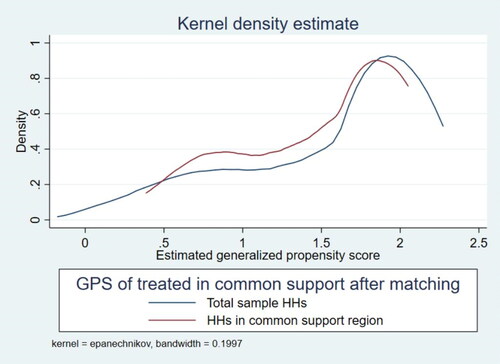
Figure 1 depicts the distribution of the treated household and the household on common support based on estimated GPS scores. As portrayed in the figure, most sampled households reside on the right side of the kernel distribution, which suggests a higher intensity of improved Coffee Arabica variety adoption.

Figure 1. GPS-score Kernel density with common support regions.

Covariate balance test

As depicted in Table 6, through the adjustment of GPS, it has been possible to improve the balance of covariates. Without the adjustment of GPS, there were significant mean differences among twelve covariates, while no significant mean difference was observed after the correction of GPS.

Table 6. Balancing: test for covariate means equality³.

Variables	T-statistics of mean difference before the match						T-statistics of mean difference After the match
	0 - 0.498753		0.512194 - 0.731706		0.737704 - 0.988048		0 - 0.498753		0.512194-0.731706		0.737704 - 0.988048
	Mean Difference	T-value	Mean Difference	T-value	Mean Difference	T-value	Mean Difference	T-value	Mean Difference	T-value	Mean Difference	T-value
Age	1.269	.599	2.403	1.237	−4.096	−1.963*	1.276	.727	2.304	1.204	−3.587	−1.708
Education level	−.311	−.558	.289	.562	−.029	−.051	.262	.525	.04747	.0907	−0.408	−.684
TLU	.150	.749	.10716	.578	−.276	−1.384	−.0817	−.456	.150	.802	−0.121	−.5729
Family size	−.934	−3.043***	.594	2.057**	.235	.740	−.171	−.54693	.427	1.548	−0.117	−.364
Distance to market	−.477	−.881	.640	1.287	−.276	−.508	.140	.31266	.58748	1.1917	−0.363	−.6268
Distance main road	1.238	2.203**	−.059	−.112	−1.168	−2.074**	−.121	−.259	.314	.623	−0.661	−1.152
Dis. iimprovseed	−1.127	−1.589	1.394	2.148**	−.512	−.716	−.343	−.631	1.1925	1.8182	−0.738	−.9951
Age square	138.71	.662	231.677	1.204	−411.272	−1.992**	110.08	.661	235.06	1.240	−347.180	−1.700
Age cube	12283.1	0.743	16723.68	1.100	−31958.1	−1.959*	7721.3	.619	17956	1.201	−25864	−1.635
TLU square	.157	.240	−.005	−.008	−.152	−.232	−.100	−.167	.081	.131	−0.036	−.051
TLU cube	.538	.224	−.240	−.108	−.256	−.106	.085	.037	−.7834	−.341	0.586	.219
Education level square	−3.178	−.465	2.763	.439	−.072	−.011	3.997	.645	−.393	−.061	−3.854	−.525
Education level cube	−15.2	−.190	19.780	.269	−8.106	−.101	52.761	.720	−12.209	−.162	−38.983	−.453
Family size square	−14.871	−3.162***	9.337	2.106**	3.886	.795	−3.026	−.586	6.865	1.598	−1.331	−.260
Family size cube	−191.8	−3.116***	120.234	2.073**	50.383	.789	−45.53	−.630	91.195	1.586	−9.775	−.141
Distance main road square	−4.313	−.633	6.817	1.088	−3.708	−.544	2.204	.374	6.081	.964	−4.870	−.654
Distance main road cube	−31.20	−.396	57.066	.787	−35.933	−.456	31.036	.443	43.8	.587	−52.895	−.601
dissorimprovseed square	−8.20	−.607	19.941	1.616	−15.259	−1.134	−3.084	−.410	18.087	1.451	−13.019	−.966
dissorimprovseed cube	19.60	.065	328.797	1.187	−406.423	−1.356	−23.097	−.224	328.35	1.187	−257.910	−.893

Note: ***, ** and * means significant at the 1%, 5% and 10% probability levels, respectively.

The dose-response function results

Once all the GPS procedures were passed, impact analysis estimated the average DRF with causal inference. The adoption intensity impact of improved Arabica coffee on household daily calorie intake per AE, Consumption expenditure and Per capita income were estimated. The average potential outcome was estimated using ten values of adoption intensity (0.1, 0.2, 0.3,… 1). The intensity of DRF adoption at level t was then calculated as E[HHExp (t)] and plotted. The estimated average impact of the adoption intensity of improved Coffee Arabica varieties was plotted against the entire adoption intensity range of the improved Coffee Arabica varieties’ distribution. Based on 100 bootstrap replications, the DRF within a 95% confidence interval was estimated. Accordingly, the model results were significant for all outcome variables, leading to the non-acceptance of all slope coefficients being zero for the null hypothesis (see Table 7). It should be noted that the computed coefficients lack a causal interpretation. On the route to causal inference, the results serve two functions, however: to create an average DRF and to reevaluate whether the covariates add bias (Hirano and Imbens, 2004; Liu and Florax, 2014).

Table 7. Consumption spending, per capita income, and daily calorie intake per AE for households are approximated using the dose-response function.

Variables	Calorie intake			Consumption expenditure			Per capita income
	Coef.	Std. Err.	t	Coef.	Std. Err.	t	Coef.	Std. Err.	t
Intensity of adoption	2401.19	2294.24	1.05	37592.08	21870.45	1.72*	−39387.47	20459.82	−1.93**
Intensity of adoption _square	−4474.76	2129.21	−2.10**	−37833.86	20297.23	−1.86*	20796.55	29252.27	0.71
GPS	−1729.51	859.08	−2.01**	−8690.44	8189.37	−1.06	14069	12534	1.12
GPS_ square	−13.14	334.44	−0.04	30.67	3188.13	0.01	−8310.92	4929.11	−1.69*
Intensity of adoption*GPS	2024.91	690.99	2.93***	1339.25	6587.14	0.20	1680.512	665.405	2.53**
_cons	3733.09	599.42	6.23***	28425	5714.15	4.97***	11195.02	8542.34	1.31
Adj R − squared	0.0998			0.0976			0.0464
Number of obs	111			111			111
Prob > F	0.0054			0.0049			0.0636

Note: ***, ** and * means significant at the 1%, 5% and 10% probability levels, respectively.

The impact of adoption intensity on daily calorie intake

There is no linear relationship between adoption intensity and household daily calorie intake per AE. The graph results suggest that at the start, the adoption intensity had a net negative impact on the daily calorie intake of the household and attained its minimum optimum level at 52.58% adoption intensity. This may be due to the fact that the adoption of improved varieties alone is not enough to achieve the desired level of yield unless full production packages (i.e., compost application rate, weed management, pruning practices, spacing practices, and shade requirement) are adopted (see Figure 2).

Figure 2. Adoption intensity on daily calorie intake dose-response and treatment effect.

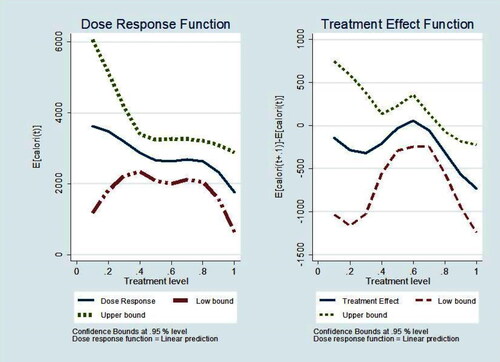
After reaching the peak at the 71.42% adoption level, the graph declines, signifying the positive impact’s intensity. It’s important not to interpret the third segment as indicating a direct cause-and-effect relationship between adoption intensity and daily calorie intake. This segment reflects wide confidence bands due to a small sample size. Approximately, 71.42% of the highest adoption level is attributed to the sample households. The GPS estimation suggests that the average optimal daily calorie intake is achieved at around 71.42% adoption intensity, with the corresponding optimum value being 2,384.80 kcal per adult equivalent. The result is similar to Kassie et al. (2014) finding in rural Tanzania. Here, the optimum level of kilocalorie intake per AE should be the primary concern.

The impact of adoption intensity on consumption expenditure

The relationship between adoption intensity and household consumption expenditure on food and drink is non-linear. Upon analyzing the graph, it becomes evident that in the initial stages, adoption intensity positively influenced household consumption expenditure, peaking at 28.41% adoption intensity (see Figure 3).

Figure 3. Adoption intensity on consumption expenditure dose-response and treatment effect.

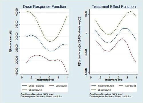
Subsequently, after reaching the optimal level, the graph exhibits a decline, signifying the negative impact of adoption intensity, with its nadir observed at 72.28% adoption intensity. However, after this dip (72.28%), the graph ascends once again, culminating in a new peak of approximately 83.66%. It’s essential to note that the third segment of the figure should not be construed as implying a causal relationship between adoption intensity and consumption expenditure. This section is characterized by large confidence bands stemming from a limited household sample. Hence, the GPS estimation result shows the average optimal consumption expenditure is attained at around 28.41% adoption intensity level, and 13,704 Birr is the corresponding optimal value. Empirical studies measuring the impacts of improved agricultural technologies on households’ consumption expenditure in Ethiopia (Kassie et al., 2014; Biru et al., 2020) confirm a positive impact between improved agricultural technology adoption and household consumption expenditure. Here, the optimum level of households’ consumption expenditures should be the primary concern.

The impact of adoption intensity on the per capita income of households

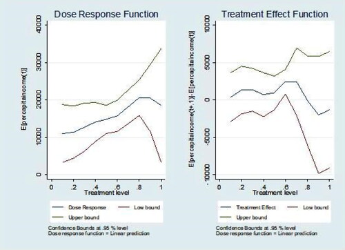
Figure 4 illustrates the influence of the adoption intensity of improved Arabica coffee varieties on the per capita income of households. As per the GPS estimation, both the per capita income and the percentage of land devoted to improved Arabica coffee cultivation rose to 74.62% and 83.66%, respectively. However, when the land utilization for improved coffee production reached 100%, the impact on income became insignificant, provided all other factors remained constant. Kassie et al. (2014) emphasized the welfare impact of improved agricultural technology adoption in rural Tanzania, while Wu (2022) confirmed the positive income impact of new technology adoption in rural China. Similarly, studies by Samuel and Beza (2019) and Muluken et al. (2021) supported the positive impact of improved agricultural technology adoption on rural farm households’ welfare in Ethiopia. Consequently, the graph shows how household income is positively impacted by the adoption intensity of improved Arabica coffee varieties.

Figure 4. Adoption intensity on per capita income dose-response and treatment effect.

Conclusion

The study’s main aim was to evaluate the impacts of adopting improved Arabica coffee varieties on farm households’ per capita income, daily calorie intake per AE, and consumption expenditure. The weak unconfoundedness assumption should be considered when the dose-response function of the generalized propensity score is estimated. Appropriate covariates were incorporated to enhance the reliability of the identification assumption and ensure the robustness of the model employed in the study. Based on 100 bootstrap replications, the DRF within a 95% confidence interval was estimated, together with the GPS estimation.

Heterogeneous effect exist among adoption levels at different doses. Three main effects were observed between improved coffee Arabica adoption intensity and daily calorie intake per AE. Initially, household daily calorie intake per AE had a negative net impact and reached its minimum optimum level at 52.58% adoption intensity, after which the impact started to inverse and attained a level of around 71.42% adoption intensity. The level of optimum adoption is 71.42%, and the household food daily calorie intake per AE is about 2,384.80 kcal per AE.

Furthermore, there were three key effects between consumer expenditure and the adoption intensity of improved Arabica coffee. Initially, household daily consumption expenditure had a net positive impact on the household’s consumption expenditure and attained its optimum level at 28.41% adoption intensity, followed by an inverse impact. The optimum level was attained at a 28.41% adoption intensity level and 13,704 Birr for the corresponding annual household consumption expenditure value. Additionally, adoption intensity had a positive impact on household income, with 83.66% representing the optimum level.

The findings of the study suggest that the adoption of improved Arabica coffee varieties tends to improve the livelihoods of adopting farmers. Importantly, increasing the intensity of adoption toward the optimal adoption level can meaningfully impact the livelihood of coffee growers in the area. In this regard, policies that improve the efficiency of coffee production and reduce the limitations of farmers’ adoption guarantee the optimum allocation of land used for superior technologies. Thus, by implementing such strategies, the livelihoods of coffee producers can be significantly improved.

Acknowledgements

We acknowledge Dilla University for financing this study. We are also grateful for the comments provided by the anonymous reviewers.

Disclosure statement

The authors declare there is no Complete of Interest at this study.

Additional information

Funding

We acknowledge Dilla University for financing this study.

Notes

1 Kebele means the smallest administrative unit of Ethiopia.

2 Ethiopian Birr is the currency unit in Ethiopia (52.13 Ethiopian Birr = 1 USD).

3 Checking the covariate balance is the main goal while estimating the GPS score. By conditioning on the estimated GPS, the study applied the method recommended by Hirano and Imbens (2004) to gauge how well covariates were balanced. The outcomes show that accounting for the GPS has significantly improved the covariate balance.

References

- Abdu, A., & Gedeo, T. A. (2013). Highland home garden agroforestry system- case study, in farmers’ strategies for adapting to and mitigating climate variability and change through agroforestry in Ethiopia and Kenya., pp. 1–15, Oregon state university, Corvallis, OR, USA.,
- Agriculture and Natural Resource Bureau Bureau. (2021). Annual report.
- Amare, M., Asfaw, S., & Shiferaw, B. (2012). Welfare impacts of maize-pigeon pea intensification in Tanzania. Agricultural Economics, 43(1), 1–14.
- Amsalu, A. (2015). Institutional context for soil resources management in Ethiopia: A review: September 2015., Addis Ababa.
- Ayele, A., Worku, M., & Bekele, Y. (2021). Trend, instability and decomposition analysis of coffee production in Ethiopia (1993–2019). Heliyon, 7(9), e08022. https://doi.org/10.1016/j.heliyon.2021.e08022
- Bia, M., & Mattei, A. (2008). A Stata package for the estimation of the dose–response function through adjustment for the generalized propensity score. The Stata Journal: Promoting Communications on Statistics and Stata, 8(3), 354–373. https://doi.org/10.1177/1536867X0800800303
- Biru, W. D., Zeller, M., & Loos, T. K. (2020). The impact of agricultural technologies on poverty and vulnerability of smallholders in Ethiopia: a panel data analysis. Social Indicators Research, 147(2), 517–544. 5-019-02166-0. https://doi.org/10.1007/s11205-019-02166-0
- CSA (Central Statistical Agency). (2015). Federal democratic republic of Ethiopia. Agricultural sample survey 2014/2015 (2007 E.C.). CSA, Addis Ababa.
- CSA (Central Statistical Agency). (2018). Reports on area and production of crops (Private Peasant Holdings, Meher Season). Addis Ababa.
- DANRB (District Agriculture and Natural Resource Bureau). (2021). District Agriculture and Natural Resources Bureau, District 4th quarter agricultural and natural resource report, 2020/21. Kochore District.
- Djebbari, H., & Smith, J. (2008). Heterogeneous impacts in PROGRESA. Journal of Econometrics, 145(1-2), 64–80. https://doi.org/10.1016/j.jeconom.2008.05.012
- GAIN (Global Agricultural Information Network). (2019). Ethiopia coffee annual report. Assessments of commodity and trade issues official U.S. government Required Report - public distribution Report Number: ET1904,
- Gao, Y., Niu, Z. H., Yang, H., & Yu, L. (2019). Impact of green control techniques on family farms’ welfare. Ecological Economics, 161, 91–99. https://doi.org/10.1016/j.ecolecon.2019.03.015
- Gelaw, F., Speelman, S., Van, H., & Van, G. (2016). Farmers’ marketing preferences in local coffee markets: Evidence from a choice experiment in Ethiopia. Food Policy. 61, 92–102. https://doi.org/10.1016/j.foodpol.2016.02.006
- Guardabascio, B., & Ventura, M. (2014). Estimating the dose-response function through the GLM approach. http://mpra.ub.uni-muenchen.de/45013/. Accessed 15 June 2017.
- Hirano, K., & Imbens, G. W. (2004). The propensity score with continuous treatments. In A. Gelman and X. Meng (Eds.), Applied Bayesian modeling and causal inference from incomplete-data perspectives.
- Hou, X. K., Liu, T. J., & Huang, T. (2020). Adoption behavior and income effects of green agricultural technology for farmers. Journal of Northwest University of Agriculture and Forestry, (Social Science Edition). 3, 121–130. https://doi.org/10.1371/journal.pone.0267101
- Houeninvo, G. H., Quenum, C. V. C., & Nonvide, G. M. A. (2019). Impact of improved maize variety adoption on smallholder farmers’ welfare in Benin. Economics of Innovation and New Technology, 29(8), 831–846. https://doi.org/10.1080/10438599.2019.1669331.
- Huang, T. T., Huang, Q. H., & Hu, J. F. (2020). Research on the impact of pilot determination on the economic benefits of family farms. World Agriculture, 9, 56–64.
- Irene, B., Aloyce, H., Elizaphan, J. O. R., & Kenneth, M. (2018). Do dairy market hubs improve smallholder farmers’ income? The Case of Dairy Farmers in the Tanga and Morogoro Regions of Tanzania, Tanzania Journal of Agricultural Sciences, 18(1), 1–12. https://doi.org/10.1080/03031853.2018.1481758.
- Kassie, M., Jaleta, M., & Mattei, A. (2014). Evaluating the impact of improved maize varieties on food security in Rural Tanzania: Evidence from a continuous treatment approach. Food Security, 6(2), 217–230. https://doi.org/10.1007/s12571-014-0332-x
- Kassie, M., Shiferaw, B., & Muricho, G. (2011). Agricultural technology, crop income, and poverty alleviation in Uganda. World Development, 39(10), 1784–1795. https://doi.org/10.1016/j.worlddev.2011.04.023
- Kippie, T. (2002). Five thousand years of sustainability? A case study on Gedeo land use. (Southern Ethiopia). Treemail Publishers.
- Kluve, J., Schneider, H., Uhlendorff, A., & Zhao, Z. (2007). Evaluating continuous training programs using the generalized propensity score. Discussion Paper No. 3255.
- Kluve, J., Schneider, H., Uhlendorff, A., & Zhao, Z. (2012). Evaluating continuous training programmes by using the generalized propensity score. Journal of the Royal Statistical Society Series A: Statistics in Society, 175(2), 587–617. https://doi.org/10.1111/j.1467-985X.2011.01000.x
- Kodama, Y. (2007). New role of cooperatives in Ethiopia: The case of Ethiopian coffee farmers cooperatives. African Study Monographs, Suppl35, 87–108.
- Li, J., & Fraser, M. W. (2015). Evaluating dosage effects in a social-emotional skills training program for children: An application of generalized propensity scores. Journal of Social Service Research, 41(3), 345–364. https://doi.org/10.1080/01488376.2014.994797
- Liu, J., & Florax, R. (2014. In 2014 Annual Meeting, July 27–29, 2014, Minneapolis, Minnesota, USA (No. 169804), USA. The effectiveness of international aid: A generalized propensity score analysis Agricultural and Applied Economics Association.
- Ma, W., & Abdulai, A. (2019). IPM adoption, cooperative membership and farm economic performance: Insight from apple farmers in China. China Agricultural Economic Review, 11(2), 218–236. https://doi.org/10.1108/CAER-12-2017-0251
- Magrini, E., & Vigani, M. (2016). Technology adoption and the multiple dimensions of food security: the case of maize in Tanzania. Food Security, 8(4), 707–726. https://doi.org/10.1007/s12571-016-0593-7
- Makate, C., Wang, R., Makate, M., & Mango, N. (2017). Impact of drought tolerant maize adoption on maize productivity, sales and consumption in rural Zimbabwe. Agrekon, 56(1), 67–81. https://doi.org/10.1080/03031853.2017.1283241.
- Mignouna, D. B., Manyong, V. M., Rusike, J., Mutabazi, K. D. S., & Senkondo, E. M. (2011). Determinants of adopting Imazapyr-resistant maize technologies and its impact on household income in western Kenya. AgBioForum, 14(3), 158–163. http://hdl.handle.net/10355/12461.
- Moat, J., Williams, J., Baena, S., Wilkinson, T., Demissew, S., Challa, Z. K. T., Gole, T. W., & Davis, A. P. (2017). Coffee farming and climate change in Ethiopia: Impacts, forecasts, resilience and opportunities. Summary report 2017. The strategic climate institutions programme (SCIP). Royal Botanic Gardens, Kew (UK). Pp. 37.
- Muluken, G. W., Jemal, Y., Getachew, S. E., Chanyalew, S. A., Dereje, K. M., & Debbebe, T. R. (2021). Adoption of improved agricultural technology and its impact on household income: a propensity score matching estimation in eastern Ethiopia. Agriculture & Food Security, 10, 5. https://doi.org/10.1186/s40066-020-00278-2
- Negash, M. (2013). The Indigenous agroforestry systems of the South-Eastern Rift Valley Escarpment, Ethiopia: their biodiversity, carbon stocks, and litterfall. [Doctoral thesis]. Tropical Forestry Reports. No. 44. University of Helsinki.
- Perfect Daily Grind. (2020). Africa coffee trade, importing, and exporting. What is the Ethiopian commodity exchange? https://www.google.com/url
- Rosenbaum, P. R., & Rubin, D. B. (1983). The central role of the propensity score in observational studies for causal effects. Biometrika, 70(1), 41–55. https://doi.org/10.1093/biomet/70.1.41
- Samuel, D., & Beza, E. (2019). Impacts of adoption of improved coffee varieties on farmers’ coffee yield and income in Jimma Zone. Agricultural Research & Technology, 21(4), 556169. https://doi.org/10.19080/ARTOAJ.2019.21.556169
- Shumete, G. (2009). Proceedings of the 16th International Conference of Ethiopian Studies, Harald Aspen. Poverty, food insecurity and livelihood strategies in rural Gedeo. The case of Haroressa and Chichu PAs, SNNP. In Svein Ege (Ed.), Birhanu Teferra and Shiferaw Bekele, Trondheim 2009.
- Solymosi, K., & Techel, G. (2019). Brewing up climate resilience in the coffee sector: Adaptation strategies for farmers, plantations, and producers. Available online at: https://www.idhsustainabletrade.com/uploaded/2019/06/Brewing-up-climate-resilience-in-the-coffee-sector-1.pdf (accessed January 24, 2021).
- Southern Nations, Nationalities, and Peoples Region (SNNPR). (2018). Regional overview. FEWSNET, USAID, Disaster Prevention and Preparedness Commission (DPPC), the Government of Ethiopia,
- Tollera, M. T. (2020). Ethiopia’s coffee-growing areas may be headed for the hills. Eos, 101. https://doi.org/10.1029/2020EO148824
- Tufaa, M., Melese, A., & Tena, W. (2019). Effects of land–use types on selected soil physical and chemical properties: The case of Kuyu District, Ethiopia. Eurasian Journal of Soil Science (Ejss), 8(2), 94–109. https://doi.org/10.18393/ejss.510744
- United Nations, Department of Economic and Social Affairs, Population Division (UNDSAPD). (2017). World population prospects: The 2017 revision, Key findings and advance tables. Working Paper No. ESA/P/WP/248.
- United States Department of Agriculture (USDA). (2020). Coffee: World markets and trade. https://downloads.usda.library.cornell.edu/usda.smis/files/m900nt40f/sq87c919h/8w32rm91m/coffee.pdf.
- World Vision. (2020). Our vision for every child, life in all its fullness; Our prayer for every heart, the will to make it so. Kochore coffee farmer’s co-operatives revitalization support project. Ethiopia.
- Wu, F. (2022). Adoption and income effects of new agricultural technology on family farms in China. PloS One, 17(4), e0267101. https://doi.org/10.1371/journal.pone.0267101
- Zhai, Z., Fuchs, A. L., & Lohmann, I. (2010). Cellular analysis of newly identified Hox downstream genes in Drosophila. European Journal of Cell Biology, 89(2-3), 273–278. https://doi.org/10.1016/j.ejcb.2009.11.012