The influence of channel morphology and hydraulic complexity on larval pallid sturgeon (Scaphirhynchus albus) drift and dispersal dynamics in the Fort Peck Segment, Upper Missouri River: insights from particle tracking simulations

Abstract

Longitudinal dispersal of migratory fish species can be interrupted by factors that fragment rivers, such as dams and reservoirs with incompatible habitats, and indirect alterations to variables, such as water temperature or turbidity. The endangered pallid sturgeon (Scaphirhynchus albus) population in the Upper Missouri River Basin in North Dakota and Montana is an example of such fragmentation and alteration due to the construction of dams. We applied a high-resolution, 2+-dimensional modelling framework composed of hydrodynamic and Lagrangian particle tracking components to simulate pallid sturgeon larval drift and dispersal along a 33-km section of the Upper Missouri River to evaluate three main issues: a comparison between multidimensional models and traditional 1-dimensional models, the sensitivity of hydrodynamics to channel morphology, and the implications of channel morphology on retention and transport-time metrics for larval fish. The results indicate that multidimensional models better represent breakthrough curves of transporting larvae compared to 1-dimensional models, especially for the long tail of slow drifters in the population. Results also indicate that channel morphology and hydraulic complexity play significant roles in larval dispersal with certain flow conditions and channel features increasing larval retention and providing potential management options to increase survival rates by adjusting flow conditions during spawning events. For example, modelling indicates increased retention times at discharges 23–38% daily flow exceedance, coincident with emergence of mid-channel sandbars. Findings additionally emphasize the need for improved understanding of biological factors that affect larval drift and dispersal.

Keywords:

• Larval dispersal
• particle tracking
• Missouri River
• hydrodynamics

Introduction and background

Longitudinal dispersal of migratory fish species can be interrupted by factors that fragment rivers, including physical barriers like dams, reservoirs that provide incompatible habitats, and indirect alterations of key variables like water temperatures or turbidity. Fragmentation affects both upstream migrating adult fish as well as downstream dispersing progeny. Managing rivers to support migratory fish often requires detailed understanding of the early-life stages during which dispersing larvae need to find supportive habitats; multiple sources of mortality during this important time period can contribute to low survival in many fishes (Mion et al. 1998; Mccasker et al. 2014; Humphries et al. 2019).

Larval drift and dispersal refer to the set of physical and biological processes that many riverine fish species undergo after spawning when embryos, free embryos (or pre-larvae, endogenously feeding on internal yolk sacs), or larvae (exogenously feeding) are entrained in the current and transported downstream. While dispersing downstream, early-life stages typically undergo morphological developments that allow them to gradually gain more control of their position in the water column, reorient themselves upstream into the oncoming current (rheotaxis), and eventually swim volitionally (Chojnacki et al. 2022). Such processes are inherently complex as the fate of dispersing larvae is a function of ontogenetic development, water temperature effects, and the flow fields encountered, which can present a wide range of turbulence, vertical shear, and flow recirculation.

Approaches to quantifying dispersal of embryos, free embryos, and larvae vary from simple hydraulic calculations, wherein advection is characterized by flow velocity and spreading of early-life stages is parameterized by a dispersion coefficient (Fischer 1973; Erwin and Jacobson 2014), to increasing hydrodynamic complexity in 2- and 3-dimensional models that incorporate variable biological realism (Garcia et al. 2013, 2015; Mcdonald and Nelson 2020; Li et al. 2022, 2023). The objective of this article is to explore how channel conditions influence larval dispersal in a natural channel. We approach this general subject by performing a case study of endangered pallid sturgeon (Scaphirhynchus albus) on the Upper Missouri River in Montana and North Dakota, USA, using a Lagrangian particle tracking model to evaluate sensitivity of larval drift and retention to river discharge, channel complexity, and hydraulics.

The Upper Missouri River and the pallid sturgeon

The Fort Peck segment of the Upper Missouri River (UPMOR) is typically defined as the segment of the Missouri River upstream from Lake Sakakawea and downstream from Fort Peck Lake in Montana and North Dakota, USA (Figure 1; Jacobson et al. 2010). The upstream part of this segment is characterized by highly altered flow regime from reservoir operations at Fort Peck Dam, including substantially decreased peak flows, decreased water temperatures (due to hypolimnetic releases), and decreased turbidity (due to sediment trapping in Fort Peck Lake) (Galat et al. 2005). The downstream 27% of the segment is influenced by the relatively natural flow and sediment regime of the Yellowstone River, which enters the Missouri about 112 km upstream from Lake Sakakawea (depending on lake level). The channel of the Fort Peck segment is mostly unaltered from its natural state with only a few instances where the banks have been stabilized for bridge crossings, boat ramps, or water intakes. The average bankfull channel width is 342 m and average channel sinuosity is 1.29 (Table A1, Appendix A). Water-surface slope of this part of the Upper Missouri River is 0.00016 (U.S. Army Corps of Engineers 2015) and the bed material is dominantly fine to medium sand with patches of gravel -and cobble-dominated substrate (Erwin et al. 2018). Under the present flow regime, the median discharge at Culbertson, Montana (Figure 1) is 263 m³*s⁻¹ (U.S. Geological Survey 2022).

Figure 1. Map showing the location of the study area (in red) within the segment of the Upper Missouri River Basin between Fort Peck Dam and Lake Sakakawea. The inset map shows the location of this area (in green) within the broader Missouri River Basin.

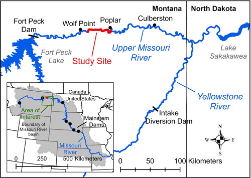
The Fort Peck segment of the Upper Missouri River and downstream portions of the Lower Yellowstone is home to a population of pallid sturgeon, an endangered benthic fish endemic to the Mississippi River basin (Jordan et al. 2016). The pallid sturgeon is a potamodromous fish that migrates 100s of km upstream to spawning sites, typically in high-velocity habitats over hard, coarse substrate (Chojnacki et al. 2020; Elliott et al. 2020). After spawning, fertilization, and incubation, free embryos hatch from eggs and begin dispersing downstream. While dispersing, the free embryos progressively develop through several temperature-mediated ontogenetic stages to achieve the ability to swim volitionally, hold themselves in the current, and begin to feed exogenously, when they are said to “settle.” Settling can take 5–13 days depending on water temperature (Delonay et al. 2016; Chojnacki et al. 2022). For the remainder of this article, we make no distinction between endogenously feeding free embryos and exogenously feeding larvae and instead refer to them collectively as larvae.

No recruitment of wild-spawned pallid sturgeon has been recorded in the Upper Missouri/Lower Yellowstone since the 1950s (Braaten et al. 2015). Lack of recruitment has been linked to high mortality during the larval drift and dispersal phase of their early life development. One plausible, popular hypothesis, the “larval drift hypothesis” (LDH), holds that the decline of the population in the Fort Peck segment results from the reduced length of dispersal distance possible between Fort Peck Dam and the headwaters of Lake Sakakawea (Braaten et al. 2012). Until recently, upstream migration of reproductive adults on the Yellowstone River has also been constrained by the Intake Diversion Dam (IDD, Figure 1); a bypass channel around IDD was completed in 2022 to allow for upstream migration and spawning on the Yellowstone River, but whether the bypass will result in recruitment has not yet been established. The LDH posits that the length of free-flowing river on either the Fort Peck segment or the Yellowstone River has been inadequate for the fish to successfully complete the larval drift phase of their early life development and that dispersal into Lake Sakakawea results in 100% mortality because of anoxic water quality conditions (Guy et al. 2015) or other sources of mortality in the headwaters.

Previous work on modelling larval dispersal

The LDH has prompted several approaches to evaluating how river management could increase survival of larval pallid sturgeons. For example, relatively simple advection/dispersion hydrodynamic transport models have been used to evaluate how many days of passive drift could be accommodated upstream from Lake Sakakawea under a range of flow and lake-extent scenarios (Erwin et al. 2018). These models used the 1-dimensional (1-D) HEC-RAS advection/dispersion model with the longitudinal dispersion parameter estimated from a dye-trace experiment. Based on a simple guideline for how many days are likely necessary for ontogenetic development of larval pallid sturgeon to reach the exogenous feeding stage, the authors concluded that the distance available was likely inadequate. A similar companion study (Fischenich et al. 2018) used different estimates of the dispersion coefficient but also concluded that few, if any, free embryos would be retained upstream from Lake Sakakawea under the assumption of passive transport. An expansion of the 1-D modelling approach linked reservoir operations, temperature-mediated larval growth rates, and additional biological assumptions about drift behaviour to evaluate effects of multiple management alternatives on pallid sturgeon populations (Fischenich et al. 2021). This study indicated that retention upstream from Lake Sakakawea was highly dependent on assumed spawning location, water temperature, and, notably, whether dispersal ends with a larval behavioural shift to rheotaxis or with initiation of exogenous feeding. The behavioural shift to rheotaxis may occur several days earlier than feeding and results in the prediction that substantially higher percentages of larvae would be retained upstream from the lake and survive to feeding (Mrnak et al. 2020). Notably, the hydrodynamic component of the Fischenich et al. (2021) model uses the built-in HEC-RAS parameterization of the dispersion coefficient based on locally derived velocity and depth (Fischer et al. 1979), modified by a coefficient to adjust calculated values to be within the range of empirical measurements made throughout segments of the model domain.

A novel study undertaken in the same river segment used a suite of acoustic Doppler current profiler (ADCP) data collected longitudinally along the channel to predict particle transport based on a 3-dimensional mapping of velocity vectors (Marotz and Lorang 2018). This model predicted there were many locations where particles would “stall” and therefore resulted in predictions of much slower dispersal and consequently higher larval survival. These authors predicted that the fastest larvae could take 31 days to transit from spawning near Fort Peck to Lake Sakakawea. Although the Marotz and Lorang (2018) model neglected continuity of mass and momentum, it indicated the value of considering channel morphological characteristics in understanding larval transport. Studies of larval transport on the Danube River, Austria, have similarly concluded that channel-morphology-mediated hydraulics are important controls on larval dispersal processes (Lechner et al. 2014, 2016).

Although 1- and 2-dimensional hydrodynamic models provide useful information on physical transport processes, they are limited by the assumptions they make regarding cross-channel and vertical velocity distributions. To address these shortcomings, fully 3-dimensional hydrodynamic models that provide a more comprehensive representation of lateral and vertical velocity gradients have also been applied to fish dispersal. A recent example of such a model being used to predict transport of invasive carp eggs on the highly engineered Lower Missouri River found that the full 3-dimensionality of the model provided additional information on the role of macroturbulence in dispersion and indicated that channel-morphological features, for example, wing dikes, can have a strong influence on interception and retention of passively drifting particles (Li et al. 2022, 2023). However, these models become increasingly difficult to implement in larger river reaches due to the need for high-resolution input data and extensive computational resources.

Although biological factors create the greatest uncertainties about larval drift dynamics in the Fort Peck segment – in particular how far upstream fish may spawn and how their progressive ontogenetic development affects probabilities of settling – additional uncertainties relate to physical processes that might be amenable to management: how do channel morphology and hydraulic complexity interact with discharge to affect interception, retention, and residence times? Improved ability to answer these types of questions would allow managers to optimize flow releases to retain larvae and to target larval sampling to explore the fate of retained larvae.

The research reported here addresses these types of questions by developing a high-resolution, 2-plus-dimensional (2+-D) particle tracking modelling framework capable of resolving hydraulic complexity including secondary flows and recirculation (Nelson and Mcdonald 1997; Mcdonald et al. 2020; Mcdonald and Nelson 2020). The “plus” in the term, 2-plus-dimensional model, indicates that the modelling approach does not fully resolve vertical components of the flow field. Nevertheless, the approach provides useful information about physical influences on dispersal processes because advection and dispersion are explicitly modelled rather than incorporated into a dispersion coefficient. The 2+-D modelling framework is also a useful compromise between computational efficiency and information content.

We address three specific research questions using this modelling approach:

• How does explicit multidimensional modelling of larval transport improve scientific understanding of dispersion processes? We evaluate this question by comparing breakthrough curves from modelled larval transport using 1-D and 2+-D approaches with results from a larval-seeding experiment.

• How sensitive are hydrodynamics of the Fort Peck segment to channel morphology? We evaluate this question by comparing dispersal-related hydrodynamics between two contrasting reaches of the river.

• What are the implications of channel morphological influences on larval dispersal, measured by retention and transport time metrics? We evaluate this question by applying a Lagrangian particle tracking (LPT) model to the contrasting river reaches.

Methods

In the following section we describe the modelling framework, consisting of a 1-D advection/dispersion model for comparison, and the 2+-D hydrodynamic model and Lagrangian particle tracking (LPT) model built on the hydrodynamic results. We then describe data collection for constructing the 33-km model domain and for calibration and evaluation of the hydrodynamic model. We follow up with a discussion of metrics that can be derived from the hydrodynamic and LPT models to evaluate sensitivity of larval dispersal to discharge, channel complexity, and hydraulics.

Modelling framework

We used an existing 1-D hydraulic and advection/dispersion model for comparison to a new 2+-D and LPT model to evaluate increases in realism associated with increased dimensionality and resolution.

1-D comparison model

The 1-D advection dispersion model used in the model comparison was developed by the U.S. Army Corps of Engineers (USACE) for the Upper Missouri River and several major tributaries in HEC-RAS (Fischenich et al. 2018, 2021). The model features cross-sections spaced every half-mile and includes a hydrodynamic component and a water quality module that can model advection-diffusion processes for arbitrary tracers through the specification of a dispersion coefficient and injection location. The hydrodynamic model was set up to simulate flows on the Upper Missouri River for July 1, 2019, by specifying discharge values measured at multiple U.S. Geological Survey (USGS) gage sites corresponding to sections between large tributary junctions. The model was then run at steady flow. The injection location was set to the closest model cross-section at rivermile 1701.31, located ∼55 meters upstream from the location where more than 970,000 larvae were released in a 2019 experiment (Braaten and Holley 2021; Braaten et al. 2022) (discussed below). The dispersion coefficient was set to 172 m²*s⁻¹ based on results from a dye tracer study performed on the UPMOR in 2016 (Erwin et al. 2018). Once the simulations had completed, breakthrough curves for the concentration of the arbitrary tracer at the nearest model transects (1691.6 and 1680.23, located ∼55 and ∼600 meters, respectively, away from the sampling stations) as a function of time were extracted from the output data for comparison with experimental larval data and 2+-D LPT simulations.

2+-D hydrodynamic model

The modelling framework used to simulate the transport of pallid sturgeon larvae consists of two components, a hydrodynamic model to simulate flow vectors and an LPT algorithm (Mcdonald et al. 2020; Mcdonald and Nelson 2020) to simulate the movement of individual particles through the modelled flow field. This LPT algorithm was developed to easily utilize outputs from the Flow and Sediment Transport with Morphologic Evolution of Channels (FaSTMECH) hydrodynamic model available within the open-source International River Interface Cooperative (iRIC) software package (Nelson et al. 2016) and was thus selected as the model to be used for this study.

FaSTMECH is a Reynolds-Averaged Naiver-Stokes (RANS) hydrodynamic model and assumes that flow is incompressible, hydrostatic, and quasi-steady (Nelson and Mcdonald 1997). The core model functionality generates 2-dimensional depth-averaged flow solutions but includes additional functionality to generate quasi-3-dimensional solutions by modelling the structure of the vertical velocity profile along the streamlines of the depth-averaged solution. The resulting solution consists of a user-specified number of vertically stacked layers of 2-dimensional flow vectors spaced logarithmically in distance from the bed that diverge from each computational cell’s depth-averaged flow vector to reflect curvature-driven secondary flows. From here on, we will refer to this approach as being a 2-plus-dimensional (2+-D) model to reflect that it falls between 2- and 3-dimensional approaches. While this approach provides a computationally efficient means to approximate the 3-dimensional flow field and secondary flows, these solutions are not fully 3-dimensional because they lack vertical flow vector components.

FaSTMECH requires input of a curvilinear computational mesh of channel and floodplain topography which can be generated within iRIC from a user-drawn channel centerline and user-specified average cell size. The topography can then be mapped to the nodes of the generated mesh by importing a digital elevation model (DEM) to iRIC and invoking an interpolation algorithm. For each modelled flow condition, FaSTMECH requires specification of parameters for the discharge in cubic meters per second ($Q$), the water surface elevation at the downstream boundary, drag coefficient ($C_d$), and lateral eddy viscosity ($\mathit{\text{LEV}}$). The drag coefficient is calibrated by iteratively running the model at incremented values to find the value that provides the best agreement between measured and modelled water surface profiles. The LEV parameter provides the user with a way to correct the calculated vertically averaged eddy viscosity to account for lateral diffusive processes.

Many models, including FaSTMECH, close the RANS equations by specifying a kinematic eddy viscosity. FaSTMECH uses a computationally efficient approach of calculating the total eddy viscosity as the sum of the calculated vertically averaged eddy viscosity with the user-specified lateral eddy viscosity. The LEV parameter thus provides a way to correct the calculated vertically averaged boundary layer eddy viscosity to account for lateral diffusive processes and can be calculated using the formula of Nelson and Mcdonald (1997): (1) $$\mathit{\text{LEV}}=\mathit{\text{CUh}}$$(1) where $C$ is a constant between 0.01 and 0.001, $U$ is mean flow velocity, and $h$ is mean flow depth. The LEV is an important parameter worthy of extra consideration and will be discussed further below because it not only influences the scaling of modelled secondary flow structures and numerical stability in FaSTMECH, but also is an input parameter to the LPT algorithm to model the turbulent diffusion of particles. Furthermore, work by Mcdonald and Nelson (2020) has shown that the above formula likely underestimates the actual value. With this consideration in mind, calculations of the LEV for this study used a value of $C$ set to the maximum value of 0.01 and the $U$ and $h$ values were extracted from the calibrated flow model after the roughness parameter had been calibrated.

Particle tracking model

The LPT algorithm of (Mcdonald et al. 2020; Mcdonald and Nelson 2020) requires a set of 2-D and 2+-D flow solutions generated from the same model run in FaSTMECH to calculate the trajectory of individual particles through the modelled reach. The algorithm provides the user with the choice of two methods to simulate particle movement: passive and active. The trajectory of passive particles is determined solely based on the advective and diffusive processes of the flow field while active particles incorporate additional biologically informed behaviours to their calculated movements. Both methods share the same governing equations for movement in the horizontal plane and only diverge in the calculation of vertical movement.

Particle movement in the horizontal x and y directions is modelled by iteratively calculating changes in particle coordinates per timestep reflecting both advective and diffusive processes as: (2) $$p_x\left(t+\Delta t\right)=p_x\left(t\right)+u\Delta t+R_1\sqrt{2D_x\Delta t}$$(2) (3) $$p_y\left(t+\Delta t\right)=p_y\left(t\right)+v\Delta t+R_2\sqrt{2D_y\Delta t}$$(3) where $p$ is the position of the particle in Cartesian coordinates, $\Delta t$ is change in time, $u$ and $v$ are the velocity components of the x and y directions, respectively, $D$ is the turbulent diffusivity coefficient, and $R$ is a random number from a standard Gaussian distribution with a mean of 0 and variance of 1. Advective processes are represented by the terms $u\Delta t$ and $v\Delta t$ while diffusive processes are modelled stochastically as a random-walk by the term $R\sqrt{2D\Delta t},$ where the turbulent diffusivity coefficient $D$ is calculated as: (4) $$D=\mathit{\text{LEV}}+\left(\beta u_{\mathrm{*}}h\right)$$(4) where $\mathit{\text{LEV}}$ is the user-specified lateral eddy viscosity, $\beta$ is an empirical value of 0.067 associated with the derived relation for vertical eddy viscosity used within FaSTMECH, $u_{*}$ is the shear velocity, and $h$ is flow depth. Values for $u_{*}$ and $h$ are updated per particle at all timesteps using values from the computational cell of the hydrodynamic model mesh that a particle is passing through at a given time.

For the passive scenario, the vertical movement of particles is calculated as a random walk similar to the formula used to define particle movement for the x and y components: (5) $$p_z\left(t+\Delta t\right)=p_z\left(t\right)+R_3\sqrt{2D_z\Delta t}$$(5)

The vertical movements of particles using the active scenario are modelled as a sinusoidal function oscillating above the bed: (6) $$S_b\left(t\right)=B+\left[\frac{A}{2}\mathrm{*}\mathrm{\text{sin}}\hspace{0.17em}\left(\frac{2\pi }{p}\right)\Delta t+\frac{A}{2}\right]$$(6) where, $A$ is amplitude, $p$ is phase, $B$ is bed elevation. The amplitude parameter controls how far above the bed a particle can move before oscillating downwards; $A$ is stipulated as a percentage of depth above the bed.

The two scenarios of vertical particle movement relate to two development phases for pallid sturgeon following spawning. Laboratory studies in quiescent water or low velocities (< 0.1 m*s⁻¹) have shown that larval sturgeon may move up and down in the water column in the initial ∼0–9 day-post-hatch (DPH) but settle to the bottom later as they develop the ability to hold themselves in the current and begin feeding (Kynard et al. 2002; Mrnak et al. 2020). These findings would suggest that the passive drift scenario might be more appropriate for the early stages of development whereas the active scenario with constrained distance above the bed might be more appropriate for post-settling dispersal. However, neither the swim-up behaviour of 0–9 DPH larvae nor the settling behaviour has been documented in hydraulic conditions that exist in the field, where strong macroturbulence is evident and mean column velocities are often in excess of 0.8 m*s⁻¹ (Erwin et al. 2018). Hence, we evaluate both scenarios as potential realizations.

Study site

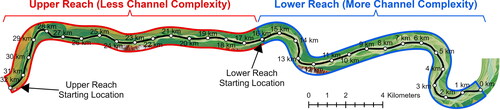
We developed a high-resolution hydrodynamic model for a portion of the Fort Peck segment that features a representative range of geomorphic and hydraulic complexity. Geomorphic classification and selection criteria for the model domain are described in Appendix A based on bankfull channel metrics. The selected model domain is 33-km long, extending from rivermile 1679 to 1701.4 and is located between the towns of Wolf Point and Poplar, Montana (Figure 1). The reach is ∼106 km (66 mi) downstream from Ft. Peck Dam, ∼155 km (97 mi) upstream from the confluence of the Yellowstone and Upper Missouri Rivers, and ∼202–232 km (126–145 mi) upstream from the headwaters of Lake Sakakawea depending on reservoir elevations. The model domain has representative ranges of channel widths and standard deviation of channel widths; it has somewhat larger valley width but a representative range of distance from the channel to valley margins; it has reaches with single-thread and multiple thread channels; the range of channel sinuosity (1–1.6) is less than some reaches that can range up to 4.9 (Table A1, Appendix A).

Field data collection and processing

Field surveys were conducted in the model reach June 5–15, 2018, September 7–8, 2018, and June 26-July 5, 2019. Measurements required for model development included: (1) detailed surveys to create a topographic surface for the hydrodynamic model mesh, (2) water-surface elevation for model calibration, and (3) discharge and velocity transects for model evaluation. All data collected during this project are archived on sciencebase.gov (Call et al. 2024).

Channel-floodplain topographic surface

Multiple sources of data were used to construct a digital elevation model of the study reach: bathymetric and terrestrial laser scanning data were collected for channel topography and previously collected airborne laser scanning data were used for floodplain topography. Bathymetric data were collected from June 6–15, 2018, and June 26-July 5, 2019, using a 210 kHz survey-grade Odom EchoTrac single beam echosounder (SBES) with an 8-degree transducer (Teledyne RD Instruments, Poway, California); shallow depths precluded use of multibeam echosounding. Boats were piloted along pre-defined transects spaced approximately 15-m from one another. Channel banks were surveyed on September 7–8, 2018, and July 3–4, 2019, using a Velodyne VLP-16 Puck 3D terrestrial laser scanner (TLS) mounted to a survey boat, accompanied by an SPG Systems Inertial Motion Unit (IMU). Positioning for SBES and TLS surveys used Real Time Kinematic Global Navigation Satellite Systems (RTK GNSS) corrections from an onshore base station. Airborne laser scanning (ALS) was collected along the Missouri River between Ft. Peck Dam and Lake Sakakawea in May 2012 by Fugro Horizons, Inc. for the USACE. These three sources of data were merged into a single digital elevation model using ArcGIS. A subsection of the DEM underlain by a hillshaded raster can be seen in Figure 2 and the spatial extent of the 2018 and 2019 surveys is indicated Figure 3. The resulting DEM and additional detailed information on the collection, processing, and editing of this data set are released in Call et al. (2024).

Figure 2. A Subset of the final channel-floodplain topographic surface. Topographic data are available in Call et al. (2024).

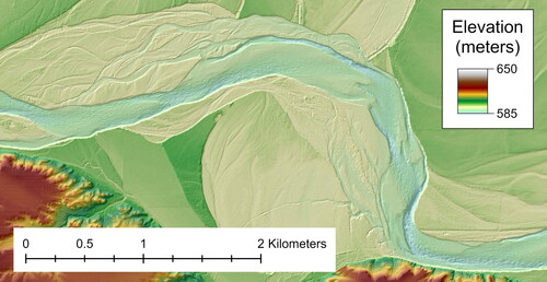
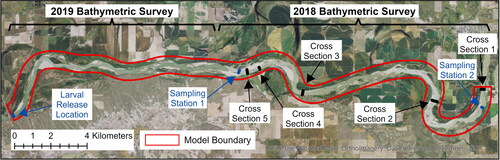
Figure 3. Map showing the locations of cross section measurements, 2019 larval drift experiment sampling stations, and the spatial extents of the 2018 and 2019 bathymetric surveys. Aerial imagery is from the USGS National Map (U.S. Geological Survey 2021).

Hydrodynamic measurements

Longitudinal water-surface profile measurements were collected using a boat-mounted RTK GNSS positioning system with measurement data collected in Hypack (Xylem Incorporated, Washington, DC). The profiles measured in 2018 were confined to a shorter length of river upstream from Poplar, Montana, compared to the 2019 measurements. The 2019 measurements were extended upstream to coincide with the spatial domain of the larval-drift experiment (described below). Independent water-surface elevation points were collected onshore using an RTK rover. The raw longitudinal profile data were manually edited to remove spurious data points generated by sudden movements associated with boat operation. Once exported from Hypack, the data were imported into ArcGIS and the elevation field compared with the nearest manual onshore water surface measurements to ensure that there were no significant errors in the boat-based measurements due to calculated offsets between the receiver and the water surface.

Discharge and velocity measurements for model validation were collected in the field on June 10, 2018, September 7, 2018, and July 1, 2019, using two Rio Grande Workhorse 1200-kHz ADCPs (Teledyne RD Instruments, Poway, California) each mounted to a USGS survey boat and georeferenced using RTK GNSS positioning systems with measurement data collected using the WinRiver 2.2 software (Teledyine RD Instruments, Poway, California). These dates were selected to approximate average discharges during the larval drift season. Five cross sections were initially established on the June 10, 2018, survey with the intention of remeasuring them during subsequent surveys (Figure 3). Due to timing and logistical constraints, only cross sections 4–5 were remeasured during the September 7, 2018, survey while only cross sections 1 and 3 were remeasured during the July 1, 2019, survey. However, three additional locations were measured on July 1, 2019, in conjunction with the larval drift experiment conducted on the same day: one measurement at the site where larvae were released and two more at each of the first two sampling locations downstream (Figure 3). A minimum of four reciprocal transects was measured at each cross section and the raw measurement data were subsequently processed using the Velocity Mapping Toolbox (VMT) (Parsons et al. 2013) to generate depth-averaged velocity profiles for use in model validation. These data are released in Call et al. (2024).

Hydrodynamic model setup

The computational mesh for the hydrodynamic model was generated as a curvilinear orthogonal grid along a user-defined channel centerline within the iRIC user-interface with a specified average cell size of 3 × 3 meters. Due to sharp bends in the channel along some sections of the reach, the specified centerline differs in many places from the actual centerline of the channel to avoid overlapping cells in the mesh. The DEM was imported into iRIC and used to interpolate elevation values to the nodes of the model mesh.

For each flow condition, FaSTMECH requires specification of a discharge, water-surface elevation at the downstream boundary, drag coefficient, and lateral eddy viscosity. Because of concerns about the quality of the June 6 and September 9, 2018, discharge measurements due to high flows on June 6 and ADCP calibration issues on September 9, we substituted discharges measured at the USGS Wolf Point, Montana streamflow gage (06177000) site just upstream of the study reach for the transect discharges. The downstream water-surface elevation was extracted by exporting the longitudinal water-surface elevation measurements from Hypack into ArcGIS and identifying the elevation of the data point closest to the downstream model boundary. We calibrated the model by iteratively running the model with incremental adjustments to the drag coefficient parameter to find the value that resulted in the minimum root-mean-square error (RMSE) value between the measured and modelled water surface profiles. Calibrated model parameters are listed in Table 1.

Table 1. Derived model parameters and the calibration RMSE for each of the three days that hydraulics measurements were taken.

Date	Discharge measured at Wolf Point gage	Downstream WSEL (m)	Roughness (Cd)	RMSE	LEV
06/10/2018	23,095 cfs (654 cms)	592.68	0.0051	0.0447	0.0469
09/07/2018	16,597 cfs (470 cms)	592.29	0.0057	0.0643	0.0343
07/01/2019	12,289 cfs (348 cms)	591.87	0.0054	0.0556	0.0259

Cfs, cubic feet per second; cms, cubic meters per second; WSEL, water surface elevation; m, meters; Cd, roughness coefficient; RMSE, root mean square error; LEV, lateral eddy viscosity.

The LEV values were calculated using Eq. (1)(1) $$\mathit{\text{LEV}}=\mathit{\text{CUh}}$$(1) with values for mean depth $h$ and mean velocity $U$ derived by fitting hydraulic geometry relations to historic channel measurements at the USGS Wolf Point streamflow gage in the form of: (7) $$h=c{Q}^f$$(7) (8) $$U=k{Q}^m$$(8) where $c,$ $f,k,$ and $m$ are parameters. 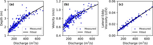Substituting these relations and their fitted parameters into the equation: (9) $$\mathit{\text{LEV}}=0.01\left(0.096Q^{0.583}\right)\left(0.108Q^{0.358}\right)$$(9) provides a simple method for initial estimations of the LEV value at any discharge for the model domain. The relations for Wolf Point are plotted with the historic field measurements in Figure 4. To evaluate sensitivity of model results to parameterization of the LEV, additional hydrodynamic simulations were run for a set of LEV values multiplied by 0.5, and 2 for use in particle tracking simulations. These different simulations will be referred to as LEVx0.5, LEVx1, and LEVx2 from here onward.

Figure 4. Historic depth (a) and velocity (b) field measurements and corresponding fitted hydraulic geometry relations used to derive a representative power-law relationship for the LEV as Eq. (9)(9) $$\mathit{\text{LEV}}=0.01\left(0.096Q^{0.583}\right)\left(0.108Q^{0.358}\right)$$(9) (c).

Hydrodynamic simulations for a range of discharges between 185 and 635 m³*s⁻¹ (approximately 80% and 20% daily flow exceedance) were run using FaSTMECH. Because this range of discharges extends below the lowest calibrated discharge, a physically based approach was needed to calculate input parameters for the downstream water-surface elevation and drag coefficient. The downstream water-surface elevations were estimated by using the existing 1-D hydrodynamic model in HEC-RAS for the Upper Missouri River (Fischenich et al. 2021) to simulate water-surface elevations for each discharge at the cross-section nearest to the downstream model boundary. These values were then adjusted to better approximate measured water-surface elevations by decreasing modelled values by 0.291 m (Figure 5a).

Figure 5. Water surface elevations derived by adjusting modeled values to better approximate measured values (a). Calibrated roughness values per discharge with Eq. (10)(10) $$\mathit{\text{Cd}}=\frac{n^{2}g}{h^{\raisebox{1ex}{$1$}\!\left/ \!\raisebox{-1ex}{$3$}\right.}}$$(10) plotted for manning’s n values of 0.028, 0.029, and 0.030 (b).

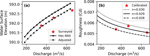
Drag coefficients were calculated by taking the relation used to calculate $\mathit{\text{Cd}}$ from flow depth and a specified Manning’s n roughness coefficient: (10) $$\mathit{\text{Cd}}=\frac{n^{2}g}{h^{\raisebox{1ex}{$1$}\!\left/ \!\raisebox{-1ex}{$3$}\right.}}$$(10) where $n$ is the dimensionless Manning roughness parameter, $g$ is acceleration due to gravity, and $h$ is flow depth, and replacing $h$ with the hydraulic geometry relation to calculate mean flow depth as a function of discharge for calculating the LEV: (11) $$h=0.0966{\mathrm{ }Q}^{0.583}$$(11)

A value of $n$ was selected by plotting Eq. (10)(10) $$\mathit{\text{Cd}}=\frac{n^{2}g}{h^{\raisebox{1ex}{$1$}\!\left/ \!\raisebox{-1ex}{$3$}\right.}}$$(10) as a function of discharge with incremental variations in $n$ together with the calibrated $\mathit{\text{Cd}}$ values plotted by discharge to find the best fit between the two (Figure 5b).

Hydrodynamic model evaluation

Comparisons of measured and modelled velocities and depths were plotted for each day and each measurement location to evaluate model performance. For comparisons of measurements made on September 8, 2018, and July 1, 2019, the modelled hydrodynamics using both the calibrated value of $\mathit{\text{Cd}}$ as well as the value derived using Eq. (10)(10) $$\mathit{\text{Cd}}=\frac{n^{2}g}{h^{\raisebox{1ex}{$1$}\!\left/ \!\raisebox{-1ex}{$3$}\right.}}$$(10) to test for sensitivity between the two; this type of analysis was not performed for measurements made on June 10, 2018, due to the calibrated and derived values for that date closely matching one another (Figure 5b). Cross sections 2 and 3 are shown in Figures 6 and 7, respectively, while cross sections 1, 4, and 5 are shown in Figures B1.1–B1.3 (Appendix B), respectively; the additional three measurements associated with the larval drift experiment are shown in Figure 8.

Figure 6. Comparisons of measured (red) and modeled (blue and black) depth-averaged velocities and depths for measurements made at cross-section 2 on June 10, 2018 (a and b, respectively), and September 9, 2018 (c and d, respectively). Solid blue lines represent values using hydrodynamics generated using the calibrated roughness parameter while the dashed black line represent hydrodynamics generated using the roughness parameter derived using Eq. (10)(10) $$\mathit{\text{Cd}}=\frac{n^{2}g}{h^{\raisebox{1ex}{$1$}\!\left/ \!\raisebox{-1ex}{$3$}\right.}}$$(10) .

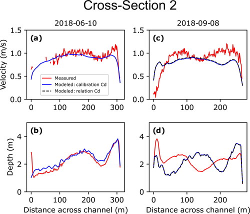
Figure 7. Comparisons of measured (red) and modeled (blue and black) depth-averaged velocities and depths for measurements made at cross-section 3 on June 10, 2018 (a and b, respectively), September 9, 2018 (c and d, respectively), and July 1, 2019 (e and f, respectively). Solid blue lines represent values using hydrodynamics generated using the calibrated roughness parameter while the dashed black line represent hydrodynamics generated using the roughness parameter derived using Eq. (10)(10) $$\mathit{\text{Cd}}=\frac{n^{2}g}{h^{\raisebox{1ex}{$1$}\!\left/ \!\raisebox{-1ex}{$3$}\right.}}$$(10) .

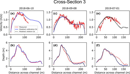
Figure 8. Comparisons of measured (red) and modeled (blue and black) depth-averaged velocities and depths for measurements made on July 1, 2019, at the larval drift experiment release site (a and b, respectively), sampling station 1 (c and d, respectively), and sampling station 2 (e and f, respectively). Solid blue lines represent values using hydrodynamics generated using the calibrated roughness parameter while the dashed black line represent hydrodynamics generated using the roughness parameter derived using Eq. (10)(10) $$\mathit{\text{Cd}}=\frac{n^{2}g}{h^{\raisebox{1ex}{$1$}\!\left/ \!\raisebox{-1ex}{$3$}\right.}}$$(10) .

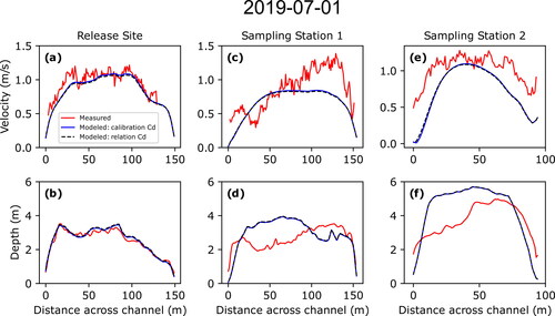
While the measurements at the five original cross-sections surveyed on June 10, 2018, show overall good agreement between measured and modelled depth-averaged velocities and depths, those resurveyed on September 8, 2018, and July 1, 2019, showed less agreement. This degradation in agreement is due to changes in bed topography that occurred between the initial bathymetric surveys during the summer of 2018 and subsequent remeasurements that are expressed as differences between the measured and modelled depths. Cross section 2 provides the clearest example of how such changes between surveys can result in mismatches between measured and modelled velocities (Figure 6). This is also evident in the three additional measurements made on July 1, 2019, as the measurement made at the larval drift experiment release location was in a location within the 2019 bathymetric survey domain and showed good agreement while the other two measurements at the first two sampling stations were within the 2018 bathymetric survey domain and showed less agreement due to changes that had occurred over the previous year (Figure 8). Cross-section 3, however, showed the least amount of difference between measured and modelled velocities for subsequent measurements due to limited changes in bed topography (Figure 7). While geomorphic change is an inherent issue in hydrodynamic modelling of dynamic sand-bedded rivers such as the Missouri River, the persistence of agreement between measured and modelled values at cross-section 3 indicates that the model maintains utility in simulating the overall velocity field even where localized channel changes may have occurred.

Comparisons of modelled velocities and depths between calibrated and derived roughness parameter values showed only very small differences (Figures 6–8). This suggests that Eq. (10)(10) $$\mathit{\text{Cd}}=\frac{n^{2}g}{h^{\raisebox{1ex}{$1$}\!\left/ \!\raisebox{-1ex}{$3$}\right.}}$$(10) provides a good approximation for calculating roughness values.

Larval drift experiment and Lagrangian particle tracking model setup and evaluation

A team of scientists from multiple government agencies conducted a larval drift experiment on the UPMOR on July 1, 2019, by releasing 771,707 1 day-post-hatch (DPH) and 200,786 5 DPH larval pallid sturgeon and sampling the water column at four different stations downstream to gain insight into fundamental questions regarding larval drift and mortality (Braaten and Holley 2021; Braaten et al. 2022). Both 1-DPH and 5-DPH fish were released simultaneously. Coordination with dam operators allowed for flows to remain relatively steady at the release location for the first ∼18 h of the experiment between 348 and 354 m³*s⁻¹. Because the release site and first two sampling stations were located within the domain of our high-resolution model, we had the unique opportunity to compare the LPT model results in the study section against the empirical larval transport data and to predictions made the 1-dimensional advection-dispersion model that had been previously developed for the Upper Missouri to predict the larval drift of pallid sturgeon (Erwin et al. 2018; Fischenich et al. 2018).

The calibrated model parameters for July 1, 2019, were used to generate hydrodynamic solutions from FaSTMECH for use with the LPT algorithm. Multiple runs of the LPT algorithm were conducted to compare results for different scenarios of vertical larval movement. One run was set to simulate vertical movement as passive drift wherein particles are distributed throughout the water column, while several other scenarios were run to simulate active drift constrained to various percentages of flow depth. Scenarios were run with LEV values of 0.5, 1, and 2 times the value derived using Eq. (9)(9) $$\mathit{\text{LEV}}=0.01\left(0.096Q^{0.583}\right)\left(0.108Q^{0.358}\right)$$(9) to evaluate sensitivity to this important parameter. Particle starting locations in the LPT model were linearly spaced at discrete points along a transect using GPS coordinates measured as larvae were released from multiple boats. 30,000 particles were simulated with a timestep of 0.1 s for 18 h of simulated time. Particle coordinates were written to output files once every 20 s of simulated time. Once particles simulations had completed, a custom Python (Python Core Team 2018) script was used to parse model outputs and extract breakthrough curves representing the number of particles as a function of time passing through spatially defined polygons located perpendicular to the direction of flow at the downstream sampling locations (Figure 3).

Effects of channel morphology on hydrodynamics and drift dynamics

We hypothesized that segment-scale GIS-scale measures of channel complexity along 0.1-mile increments of river (Table A1, Appendix A) are indicative of hydraulic complexity that is relevant to dispersal of larval sturgeon. To evaluate channel morphological controls on hydraulic complexity and larval transport, interception, and retention, we divided the model domain into contrasting upper and lower reaches (Figure 9). The lower reach is notable for having somewhat higher bankfull channel width and higher sinuosity (Table A1, Appendix A), which we hypothesized would lead to overall greater hydraulic complexity. Because the bankfull measures of channel complexity seemed to underestimate field-observable characteristics, we also considered the number of channels evident during low-flow conditions as documented in the lowest modelled discharge. The average number of channels in the low-flow condition for the lower reach is 2.3 while that for the upper reach is 1.7 (Table A1, Appendix A).

Figure 9. Map of the model reach showing the spatial extent of the upper reach (red) and the lower reach (blue) and their respective starting locations for Lagrangian particle tracking (LPT) simulations in addition to the channel centerline and reference points per kilometer from downstream to upstream used to identify general locations within the study reach.

Three different vertical movement scenarios were used for each upper and lower reach simulation for each discharge: passive movement as a random walk throughout the water column (passive), active movement constrained to the bottom 75% (active75pct), and bottom movement constrained to the bottom 60% depth (active60pct). The values of 75% and 60% were selected based on results from the drift experiment comparison that found these values to best match 1-DPH and 5-DPH larvae, respectively (discussed below). To ensure that particle starting locations were in sections with similar channel widths, we identified starting channel locations with approximately 120 m widths. To ensure both sub-reaches maintain the same length, the bottom 1.25 km of the total model reach was excluded from analysis. 30,000 particles were run for each discharge for a simulated duration of 36 h using a timestep of 0.1 s with outputs written every 10 s. While experimentation with different timesteps showed very minor sensitivity to results, the value of 0.1 s was selected as it allows for several random walk iterations as particles transverse each cell (Eqs. (2)(2) $$p_x\left(t+\Delta t\right)=p_x\left(t\right)+u\Delta t+R_1\sqrt{2D_x\Delta t}$$(2) , (3)(3) $$p_y\left(t+\Delta t\right)=p_y\left(t\right)+v\Delta t+R_2\sqrt{2D_y\Delta t}$$(3) , and (5)(5) $$p_z\left(t+\Delta t\right)=p_z\left(t\right)+R_3\sqrt{2D_z\Delta t}$$(5) ) while also allowing for reasonable simulation times. Simulations were additionally run using LEVx0.5, LEVx1, and LEVx2 values to test for parameter sensitivity. Animations of all LEVx1 simulations are available in Call et al. (2024).

Larval dispersal metrics and analyses

We extracted data from model runs to calculate metrics related to larval dispersal. The analyses focus on bulk hydraulics (medians and inter-quartile ranges (IQRs) of velocity, depth, and width), derivative hydraulics (helix strength, emergent bar features, and total wetted perimeter), and LPT particle metrics (particle retention, mean residence time, mean transit time) to evaluate sensitivity of larval dispersal to discharge and channel morphology. The analyses are intended to improve understanding of dispersal dynamics for application to flow management and larval sampling strategies.

Results from the upper and lower reach runs were post-processed using a custom Python script to calculate metrics for average hydraulics, particle retention, and particle transport time. Hydraulic variables were medians and IQRs of velocity magnitude, depth, and channel width, and mean helix strength. Helix strength was measured as the difference in angle between the surface and near-bed velocity vectors, an indicator of secondary flow. In addition, we calculated hydrodynamically derived geomorphic variables as functions of discharge, including total wetted perimeter and number of emergent features. Emergent features are dry polygons (mid-channel bars and islands) within the wetted channel and entirely surrounded by water.

Metrics derived from the LPT indicate how passively dispersing particles would be affected by discharge, channel morphology, and hydraulics. The percent retained metric is the number of particles that have been retained upstream of the downstream boundary of the model by the end of the 36-h simulation divided by the total number of particles released. The residence time metric is the average time that all 30,000 of the released particles spent in transport before exiting the downstream boundary over the 36-h simulation. The transit time metric is the average time for only those particles that have exited the downstream boundary by the end of the 36-h simulation. Residence time and transit time metrics provide slightly different information on particle retention during each simulation. Specifically, high-retention locations exist in each of the hydrodynamic solutions where particles can become trapped permanently, a condition that can obscure attempts to calculate the average time for particles to exit the reach for those that are not permanently retained. Therefore, the two parameters together provide a clearer description of transport and retention processes.

We used non-parametric Kruskal-Wallis tests to evaluate whether distributions of hydraulic variables (depth, velocity, helix strength, channel width) in upper and lower reaches and at identical discharges were likely from the same populations. We illustrated variability in those distributions by graphically comparing how IQRs varied with discharge. For depth, velocity, and helix strength each dataset in each reach consisted of approximately 500,000 points. For channel widths, which were evaluated on a cross-section basis, each dataset had approximately 5,000 values. We limited statistical analyses of emergent features, wetted perimeter, and dispersal metrics to graphical comparisons as functions of discharge, consistent with an exploratory approach.

Results

Our analyses address three questions related to hydraulic complexity and larval drift dynamics. First, to evaluate the relative information content of different modelling approaches we compare 1-D advection/dispersion and 2+-D LPT breakthrough curves (passive and active) with experimental larval drift data. This comparison assesses additional information and realism gained by increasing the dimensions and resolution of dispersal modelling. Second, we extend evaluation to channel-morphological variation in hydrodynamics by comparing hydraulic metrics for the contrasting upstream and downstream reaches. This evaluation intends to quantify the effects of increasing channel complexity on hydraulic metrics related to larval retention. Third, we assess the realism of LPT results for both reaches by calculating biologically relevant metrics (for example, residence time, transit time). Evaluation of these metrics is intended to explore how dispersal of passively transported larvae will be affected by channel complexity and discharge variation.

Comparison of modelled breakthrough curves with experimental data

2+-D LPT and 1-D advection/dispersion breakthrough curves and larval catch data for sampling stations 1 and 2 indicate relative performance of the models to actual dispersal data (Figure 10). Each dataset was placed on different y-axes scaled to each dataset’s minimum and maximum values since the primary focus of this analysis was on the timing differences as many uncertainties in the larval sampling process preclude meaningful comparison between the number of particles passing through each station and the number of larvae sampled. The 1-D advection/dispersion breakthrough curves are notably more symmetric than the LPT and experimental data, which show asymmetry indicative of a rapid arrival front followed by a slow tail. Based on fitting by eye, we found that the best agreements in timing and width of the curve between the LPT models and larval data were the active75pct for 1 DPH larvae and active60pct for 5 DPH larvae overall between both sampling stations. Fitting by eye was an appropriate approach given the fragmentary nature of the actual catch data (Braaten and Holley 2021). Active particles constrained to the bottom 75% of flow depth arrived at the first and second sampling stations 0.71 and 1.3 h, respectively, after passive particles while active particles constrained to the bottom 60% of flow depth arrived at the same sampling stations 0.96 and 1.8 h, respectively, after passive particles.

Figure 10. Comparisons of breakthrough curves from the 1-dimensional (1-D) model, Lagrangian particle tracking (LPT) simulations, and larval catch field data for 1-day-post-hatch (DPH) larvae at stations 1 and 2 (a and b, respectively) and 5-DPH larvae at stations 1 and 2 (c and d, respectively).

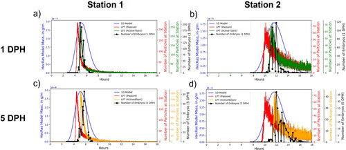
The sensitivity of the modelled breakthrough curves to LEV values was evaluated by plotting the field data and modelling data together and comparing the overall shapes of the curves. We compared LEV values 0.5, 1, and 2 times the base value for active75pct and passive particles (LEVx0.5, LEVx1, and LEVx2, respectively, Figure B1.4, Appendix B) and for active60pct and passive particles (Figure B1.5, Appendix B). This analysis shows that differences in the LEV value changed the height and width of the resulting breakthrough curves. Generally, higher LEV values result in greater longitudinal dispersion with wider and shorter curves while smaller values result in lower longitudinal dispersion with narrower and taller curves. The comparison between particles and the number of larvae passing each sampling station strongly indicate that the width and tail of the curves in the LEVx0.5 and LEVx1 particle scenarios are better fit to the larval catch data than the LEVx2 particle scenario. This is evident for LEVx2 particle scenarios at the second sampling station where the tail of the curve for the number of larvae decreases much faster than for the particles (Figures B1.4f and B1.5f, Appendix B). While LEVx0.5 appears to match the width of the curve slightly better than LEVx1, definitively identifying either as a better fit with the larvae is more difficult because the differences between them are less pronounced than with LEVx2 and uncertainties associated with sampling could result in the actual tail of the distribution being underestimated.

The 1-dimensional model shows good agreement with larvae in terms of the timing of peak concentrations, but substantially overpredicts dispersion at station 1 for both 1 and 5 DPH larvae. The LPT particle tracking model performs better at capturing the shape and width of the distributions, particularly the long tail of the distribution, which represents slower drifting larvae.

Hydraulic and geomorphic comparison of upper and lower reaches

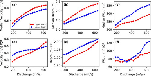
Comparing the medians of velocity (magnitude), depth, and width with discharge between the two reaches (Figure 11a–c) shows that the upper reach is generally faster, deeper, and narrower while the lower reach is generally slower, shallower, and wider. P values for the Kruskal-Wallis tests are uniformly ≪ 0.01. The IQRs of the same variables show more complex patterns than for the medians (Figure 11d–f). The lower reach has a higher variability and therefore higher IQRs of velocities below 455 m³*s⁻¹ but is surpassed by the upper reach above that discharge. While median depths at discharges are greater in the upper reach, the IQRs of depths are greater in the lower reach. The IQRs of widths are larger in the lower reach except for discharges ranging 305–395 m³*s⁻¹ where upper and lower IQRs are comparable.

Figure 11. Comparison of median values of velocity, depth, and width (a, b, and c, respectively) and inter-quartile ranges (IQR) for velocity, depth, and width (d, e, and f, respectively) for the upper reach (red) and lower reach (blue).

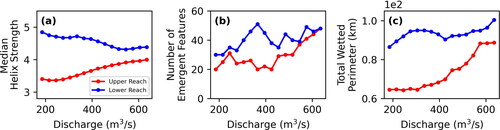
The values for median helix strength, total number of emergent features, and total wetted perimeter are larger for the lower reach for all discharges and indicate greater channel complexity (Figure 12a–c, respectively). Similar to other hydraulic variables, the Kruskal-Wallis tests for helix strength distributions between the reaches have p values ≪ 0.01. Greater helix strength across discharges indicates greater secondary flows with the potential to advect particles from the thalweg and into channel-marginal locations for interception and retention. More emergent features indicate greater hydraulic complexity and number of transport pathways around islands and exposed mid-channel sandbars; this effect is especially pronounced in the lower reach with a peak at 360 m³*s⁻¹. Greater total wetted perimeter indicates more bank length and shoreline complexity to accommodate interception and retention along the channel margin.

Figure 12. Comparison of median helix strength (a), number of emergent features (b), and total wetted perimeter (c) for the upper reach (red) and lower reach (blue).

LPT comparison of upper and lower reaches

The 2+-D LPT model results document variation of retention, mean residence time, and mean transit time with transport scenario (passive, active75pct, or active60pct) and between upper and lower reaches. Generally, retention, mean residence time, and mean transit time all decrease with increasing discharge (Figure 13a–c). All three metrics generally decrease as transport scenarios progress from active60pct, active75pct, to passive transport. That is, particles confined to lower portions of the water column encounter lower velocities and move more slowly through the channel. In addition, particles are generally slower in the lower reach compared to the less-complex upper reach. However, deviations from these general trends are evident in the active60pct particles as there is much more variability between the two reaches at flows greater than 395 m³*s⁻¹ for the percent of particles retained and mean residence time metrics and for flows greater than 305 m³*s⁻¹ for mean transit time. This is due to a few powerful eddies located in the upper reach that release very few intercepted active60pct particles once intercepted, particularly at kilometre 18 along the centerline (see upper reach animations in Call et al. (2024); locations of specific features are provided in a local addressing system). We interpret this to result from secondary flow vectors at depths where particles are directed towards the centre of the eddies. This influence might be exaggerated by the model assumption that larvae would continue to be trapped at depth in the eddy rather than be transported closer to the surface by macroturbulence. Nevertheless, retentive eddies appear to be systematically associated with flow separation at downstream tails of bars and in downstream parts of secondary channels, which are in fact salient features of the channel.

Figure 13. Each of the three vertical movement scenarios (passive is red, active75pct is blue, and active50pct is green) for the percent of particles retained for the upper and lower reaches (a and b, respectively), mean residence time for the upper and lower reaches (c and d, respectively), and mean transit time for the upper and lower reaches (e and f, respectively).

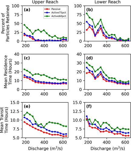
Similarly, particle retention and mean residence time increase substantially and then decline for all transport scenarios for lower-reach particles in the range 305–365 m³*s⁻¹. This deviation from the general monotonic decline of retention and residence time with increasing discharge is indicative of hydraulic complexity that emerges at this specific range of discharges as channel features such as sandbars begin to be overtopped by shallow flows.

Plotted functions for both the percent of particles retained and mean residence time as a function of discharge (Figure 13a–d) are biased by the extremely long residence time of particles that are trapped beyond the 36-h simulation. In contrast, the mean transit time functions (Figure 13e and f) count the residence time only for those particles that exit the model domain during the simulation. The mean transit time functions show the same decrease in particle velocity from passive to active75pct, but the contrast between the upper and lower reach is not as great. For passive particles, transit times in the lower reach between 215 and 365 m³*s⁻¹ are less than those in the upper reach, but greater at 185 m³*s⁻¹ and in the range of 395–605 m³*s⁻¹. Active75pct particles follow a similar pattern to passive particles, but with more variability as a function of discharge. While the mean transit time functions also show a decrease in particle velocity from active75pct to active60pct, the contrast between the upper and lower reaches is much more complex due to increased retention of active60pct particles as presented above. Transit times are greater in the upper reach between 185 m³*s⁻¹ and 335 m³*s⁻¹, then switch place with transit times in the lower reach being greater between 365 m³*s⁻¹ and 395 m³*s⁻¹, before increasing in the upper reach again over the lower reach above 425 m³*s⁻¹ and higher. The comparison indicates that the transit time functions are a broad measure of advection whereas the retention and residence time functions emphasize the potential for some particles to get retained for longer times, effectively increasing dispersion.

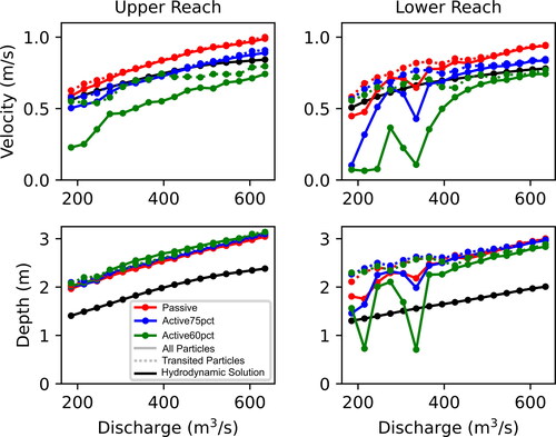
In contrast to the hypothesis that retention, residence time, and transit time should be greater in reaches with increased geomorphic and hydraulic complexity, transit times for passive and active75pct particles in the upper reach are greater than in the lower reach at discharges between 215 and 365 m³*s⁻¹ (Figure 13f). However, analysis of the velocities and depths experienced by each particle involved in these calculations provides additional insight (Figure 14a–d). Velocity values calculated for transited particles are higher in all cases than those calculated for all particles for each transport scenario. While median velocity and depth values for transited particles show increasing monotonic relationships in the upper reach, elevated values in the range of 215–365 m³*s⁻¹ are seen in the lower reach, the same discharge range that transit times were also elevated in the lower reach. Thus, while many particles are being retained, those that can exit the system are traveling slightly faster than the median velocity. This indicates that there are substantive differences in hydraulic variables between advection and retention pathways that vary with discharge. While the overall velocity may be lower at low flows, those particles moving through the system tend to travel through transport pathways that are faster and deeper. Such pathways can emerge due to flow constrictions created by flow being routed through sections of channel that are narrower at lower flows. Examples of such pathways can be observed for low flows at kilometres 7.8, 13, and 14.4 in the accompanying animations (Call et al. 2024).

Figure 14. Median velocities (a and b) and depths (c and d) in the upper reach (a and c, respectively) and lower reach (b and d, respectively) for all particles (plotted as solid lines) and only those that exit the reach (plotted as dashed lines). Lines are colored according to the method of vertical movement (passive is red, active75pct is blue, active60pct is green). The black solid lines are the median velocities and depths calculated from hydrodynamic solutions for each reach.

Results discussed above apply specifically to LEVx1 simulations. The LEV sensitivity analysis showed that while LEVx0.5 simulations resulted in greater retention and longer residence times compared to LEVx1 and LEVx2 simulations, these changes were generally consistent between both reaches and vertical movement scenarios. Regardless of LEV, the lower reach had overall greater retention and longer residence times compared to the upper reach (Figures B1.6 and B1.7). Differences in LEV values resulted in complex but minor changes to transit times with increasing variability as particles were constrained closer to the bed (from passive to active75pct, to active60pct, Figures B1.8a–c, respectively, for LEVx0.5, B1.8d, e, f, respectively, for LEVx1, and B1.8g, h, and I, respectively, for LEVx2). These differences are likely due to the LEV’s complex influence on particle retention and to the fact that the transit time metric calculation excludes retained particles. Adjusting the LEV in hydrodynamic simulations can result in differences to the size, shape, and vector orientations of eddies and other secondary flow features that intercept particles; adjustments to the LEV in the LPT change the probability of an intercepted particle breaking free due to the LEV controlling the dispersion distance that an intercepted particle can move at each time step.

Discussion

Downstream dispersal of early life stages of many fishes is complex and governed by interactions of diverse factors including hydraulics, water temperature, ontogenetic development pathways, food availability, and predation. Our objective is to increase predictive understanding of physical dispersal processes for pallid sturgeon free embryos and larvae in a river segment that has had no documented recruitment to the population in over 70 years. Our emphasis is on the roles of channel morphology and hydraulic complexity as factors in mediating dispersal, with the intent that improved understanding will provide additional options for river and species management. Additionally, this analysis is intended to document the utility of improved modelling tools in supporting management decisions.

Our modelling approach is based on the premise that increased physical realism achieved by using a high-resolution, multidimensional hydrodynamic model coupled with a Lagrangian particle tracking model will provide insights into the physical processes governing transport and fate of larvae. The modelling approach is certainly not complete as hydraulics are simplified to a quasi-3-dimensional or 2-plus-dimensional approach (2+-D) while also neglecting water temperature and the gradual acquisition of volitional swimming – factors that are known to affect dispersal rates. Nevertheless, this approach provides insights that are relevant to management. In particular, our analyses indicate:

• the value added by multidimensional models in demonstrating the high skew of physically based breakthrough curves – favouring a long tail of slowly drifting larvae – compared to 1-D advection/dispersion models with dispersion coefficient parameterization;

• active vertical movement methods provided better fits with 1 and 5 DPH larvae suggesting that purely passive assumptions may not be appropriate and support the idea that larvae are able to continually slow their movement in the flow and hold themselves closer to the bed as they grow and develop;

• functional relations between discharge and residence (and transit) times, which indicate how management of discharge through reservoir releases may be used to increase retention of larvae;

• spatial relations between measures of channel complexity and dispersal metrics, indicating where larvae may be retained and therefore efficiently sampled to evaluate sources of mortality.

The 2+-D LPT breakthrough curves conform better to experimental larval catches compared to the 1-D advection/dispersion model (Figure 10). Further, the 2+-D LPT computations show substantially increased skewness toward a long tail of slowly drifting larvae compared to the 1-D advection/dispersion model.

These results are supported by observations from laboratory mesocosm studies of pallid sturgeon larvae that have shown a gradual transition from passive to active drift in the days after larvae hatch as morphological developments allow them to gain greater control against the current (Kynard et al. 2002; Mrnak et al. 2020). The improved fit of the model to larval results when using active assumptions supports the idea that the movement of 1 DPH larvae is not completely passive because by that time the larvae might have some volitional swimming abilities providing resistance against the current or localization of drift at greater depths where velocities are lower, although they are still being transported through most of the water column. The agreement of LPT results with active movement in the bottom 60% of the water column with 5 DPH breakthrough curves aligns with mesocosm and field study observations that older larvae are able to continually slow their movement in the flow and hold themselves closer to the bed as they grow and develop (Braaten et al. 2008, 2010; Mrnak 2019).

The differences between the outputs between the 2+-D LPT and 1-D advection-dispersion highlight the utility of the more complex model in resolving dispersal processes important to management decisions. In particular, the 1-D advection-dispersion model over predicts dispersion, especially underestimating the cohesiveness of the leading front of the particles. Moreover, explicit modelling of dispersion in the 2+-D LPT predicts long tails of slower moving larvae, consistent with experimental results and potentially important in predicting probability of survival. The spatially explicit output from the 2+-D LPT also provides insight into where particularly long retention might occur and where, therefore, sampling to evaluate growth and survival would be most effective.

Although the 1-D modelling approach has been shown to be of value in evaluating reservoir management alternatives (Erwin et al. 2018; Fischenich et al. 2021), distillation of dispersion processes into a single coefficient de-emphasizes the potential contribution of the slow drifters to the population. Notably, the fate of slow drifters remains uncertain: although it has been assumed that larvae retained upstream of Lake Sakakawea headwaters will not perish from anoxia (Guy et al. 2015), there may be other sources of mortality.

Analysis of hydraulic variables by reaches with contrasting channel morphology and hydraulic complexity indicates that segment-scale geomorphic metrics are predictive of hydraulic conditions. Hydraulic analyses confirmed that the lower reach with somewhat greater bankfull width, slightly greater bankfull sinuosity, and higher number of low-flow channels had lower median velocities, shallower median depths, and greater median widths over a wide range of discharges (Figures 11 and 12; Table A1, Appendix A). In addition:

• Mean helix strength was greater in the lower reach, indicative of higher potential for secondary flows that may transport larvae to channel-marginal locations. The highest mean helix strengths were associated with discharges less than 400 m³*s⁻¹, about 17% daily flow exceedance.

• Mid-channel bars and islands were more numerous in the lower reach, indicative of greater numbers of flow paths and consequent hydraulic complexity. The distribution of emergent features with discharge has a modal peak at 360 m³*s⁻¹, indicating that reservoir releases targeting that discharge may increase larval retention.

• Total wetted perimeter is greater in the lower reach over the entire range of discharges modelled, indicating greater potential shoreline habitat availability.

The LPT model provided a means to translate 2+-D hydrodynamics into metrics that are more directly linked to larval transport and fate. Notably, the relations of discharge to percent particle retention, mean residence time, and mean transit time all showed decreasing retention with increasing discharge. Particles that were modelled as actively moving within 60% of the bottom of the river predictably had the highest retention, followed by those that moved actively within 75% of the bottom and those that were modelled as passively distributed throughout the water column (Figure 13). These results indicate the importance of improving biological understanding of how larvae move in the water column during ontogenetic development. Gradual acquisition of rheotactic behaviour (Mrnak et al. 2020) exposes larvae to lower velocities in general.

With few exceptions, the movement of modelled larvae through the model domain was slower in the lower reach compared to the upper. One exception is evident in percent retention and mean residence time at discharges greater than 400 m³*s⁻¹, where particles in the upper reach move more slowly than the lower reach (Figure 13a,b). This anomaly apparently results from a few very retentive eddies in the upper reach (notably at kilometre 18 along the centerline; Call et al. (2024), animations). Additional anomalies from the monotonic decline of retention metrics with discharge are evident in percent retention and mean residence time for the lower reach at discharges 300 – 360 m³*s⁻¹. Similarly, these anomalies seem to be associated with specific hydraulic conditions that are actualized at that range of discharges. Understanding where and when such anomalies might occur could provide guidance for reservoir releases, perhaps to identify an optimal discharge that would increase retention.

Comparison of LPT results with larval catch data suggest that the appropriate value of LEV lies within the range of LEVx0.5 and LEVx1 and that LEVx2 values resulted in breakthrough curves that were too wide compared to actual dispersion. While decreasing the LEV from the baseline condition results in an overall increase in the percent of particles retained and mean residence times, changes in the LEV result in complex changes in the mean transit time due to changes in which particles are retained and therefore not included in transit time calculations. More work is needed to better understand this parameter and the appropriate range of values for use in different rivers.

The comparison between mean residence time and mean transit time emphasizes the importance of locations along the channel where particles tend to be trapped for long times. To some extent, the trapping of particles might result from the inability of the model to generate vertical components of turbulence, which would tend to move particles higher in the water column and allow for more exchange with the main current. On the other hand, the modelled conditions that result in long residence times result from realistic hydraulics inherent in the channel geometry. Specifically, visual examination of the animations indicates that highly retentive eddies tend to exist at downstream ends of mid-channel bars, in the downstream ends of secondary channels, and in alcoves along the bank. Hence, while the model might over predict residence time in these traps, their existence is real and the ability to identify these locations is an important feature. This type of analysis could guide sampling designs to evaluate whether trapped larvae are likely to survive or, instead, subject to enhanced mortality due factors like excessive turbulence, predation, or lack of food.

Superficially, the trapping locations identified in our model appear similar to the “stall” locations identified by Marotz and Lorang (2018) based on extrapolation from ADCP measurements without applying conservation of mass or energy to transport calculations. Marotz and Lorang (2018) calculated that the vast majority of drifting larvae at ∼287 m³*s⁻¹ would be advected to channel margins and stall, resulting in a travel time of 31 days for the fastest particles for the entire Fort Peck segment, which would be more than sufficient for development of larvae to settlement and first feeding. Our 2+-D hydrodynamic and LPT model at 275 m³*s⁻¹ indicates that the vast majority of particles transit rapidly through the model domain (Call et al. (2024), animations) and that only 6–39% of particles for LEVx1 scenarios and 26–57% of particles for LEVx0.5 scenarios would remain in each 16-km sub-reach after 36 h. Nevertheless, both our model and Marotz and Lorang (2018) support the idea that physical processes will create a long tail of slow drifters, either few (as in our model) or many (as in Marotz and Lorang). Because no recruitment of pallid sturgeon has been documented in this river segment for 70 years, either there is another, undocumented source of mortality, or, as other authors have argued, the vast majority of drifting larvae end up succumbing to anoxia in Lake Sakakawea (Braaten et al. 2012; Braaten and Holley 2021).

Our modelling results indicate factors that might speed or slow dispersal of pallid sturgeon larvae in the modern river in which the spring peaks in the flow regime have been substantially decreased relative to the natural condition (Delonay et al. 2016). The highest discharge we modelled (635 m³*s⁻¹) is below flood stage, generally within the banks, whereas floodplain-connecting flows would be expected annually in the unaltered river. Under that more-natural hydrologic condition, hydraulic roughness created by floodplain vegetation might have had a strong effect on slowing downstream larval dispersal (Coutant 2004). Floodplain-connecting flows are generally avoided under present-day management decisions because of the socio economic costs (U.S. Army Corps of Engineers 2021).

Summary and conclusions

We developed a high-resolution 2+-D hydrodynamic model coupled to a Lagrangian particle tracking model (LPT) for a representative 33-km section of the Upper Missouri River in Montana and North Dakota, USA. We used the coupled models to evaluate the extent to which channel morphology and hydraulic complexity mediate transport and fate (dispersal) of early-life stages of the endangered pallid sturgeon. Whereas the prevailing modelling approach uses 1-D hydraulic models with advection/dispersion transport components parameterized with a longitudinal dispersion coefficient, the 2+-D LPT model simulates the physical processes that are responsible for dispersion. Breakthrough curves of simulated transported particles with the 2+-D LPT model are characterized by steep arrival and long, skewed tails of slow drifters whereas the 1-D breakthrough curves are more symmetrical and fail to predict the long tails. Comparison with samples from a larval-release experiment demonstrate that the 2+-D LPT results are more realistic, especially when using transport scenarios with larval particles confined to within 60% of the depth above the bed.

When applied to two reaches within the model domain with contrasting channel complexity, the 2+-D model predicts substantial hydraulic variation between the low- and high-complexity reaches, including lower mean velocities, shallower mean depths, and wider mean channel widths in the high-complexity reach. Hydrodynamic model results also documented higher helix strength, a larger number of mid-channel bars and islands, and higher total wetter perimeter, all indicative of greater hydraulic complexity that could lead to increased retention of drifting larvae.

When coupled with the LPT, model results produce metrics that relate more directly to larval retention, including percent retained after the 36-h simulation, mean residence time in the model domain, and mean transit time. Each of these metrics decline with increasing discharge but anomalies from the monotonic decline indicate discharges and locations where particles get trapped into longer residence. Generally, transport scenarios with particles passively distributed in the water column show higher particle velocities, shorter residence times compared to those constrained to active transport patterns at 60–75% depth above the bed.

The 2+-D LPT model results provide key insights into the potential for slow drifters to persist longer in the Upper Missouri River. The retention-discharge functions show specific discharges that could be targeted in reservoir releases to optimize retention. Moreover, the identification of morphologically controlled locations of high residence time within the model domain provides guidance for larval sampling to evaluate the fate of slow drifting larvae. In general, these results indicate that the increased information content provided by high-resolution hydrodynamic modelling, coupled with Lagrangian particle tracking, may be a useful tool to understand downstream dispersal of early-life stages of fish, which is a critical management concern.

Acknowledgments

We thank and acknowledge the contributions of Patrick Braaten through his leadership in planning and executing the 2019 Upper Missouri River larval drift experiment. We also thank Brian Anderson, Casey Hickcox, Edward Bulliner, Maura Roberts, and Tyrell Helmuth for their efforts in field data collection. Any use of trade, firm, or product names is for descriptive purposes only and does not imply endorsement by the U.S. Government.

Disclosure statement

No potential conflict of interest was reported by the authors.

Data availability statement

All data used in this analysis are cited and available in sciencebase.gov (Call et al. 2024).

Additional information

Funding

This research was jointly funded by the US Geological Survey Ecosystems Mission Area, Species Management Research Program and the US Army Corps of Engineers, Missouri River Recovery Program.

Notes

1 River miles are the customary units for referencing locations along the Missouri River. River miles start at zero at the confluence of the Missouri River with the Mississippi River at St. Louis. River miles are retained here to clarify communications with resource management agencies. River miles can be converted to river kilometers by multiplying by 1.601.

Appendix A.

Geomorphic classification of the Fort Peck segment, Upper Missouri River

Considerable investment in data collection is needed to construct hydrodynamic models that are of sufficient spatial resolution to answer the questions posed at the outset of this study and are also sufficiently calibrated over a relevant range of flow exceedances. A fundamental question is how well a reach selected for high-resolution hydrodynamic modelling represents the hydraulic variability inherent in longer segments of rivers. The location of the Upper Missouri River (UPMOR) hydrodynamic model domain was a trade-off between logistics (access to boat ramps, coordination with a live larval drift experiment) and the desire to capture geomorphic and hydraulic variation representative of the Fort Peck to Lake Sakakawea segment (Figure A1). To address representativeness, we evaluated geomorphic variability in the Fort Peck Segment, UPMOR. The longitudinal geomorphic classification shown here is documented in greater detail in Jacobson et al. (2023a) and digital datasets are available in Jacobson et al. (2023b).

Figure A1. Location map showing the Upper Missouri River study area.

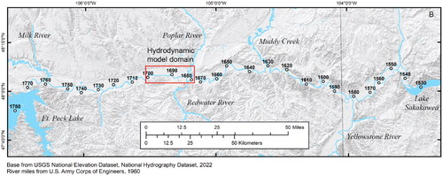
Approach and methods

We developed geographic information system (GIS) datasets for geomorphic variables that were considered useful descriptors of bankfull channel complexity. We used 2019 aerial photography (United States Department of Agriculture 2019) to digitize the bankfull channel boundary identified as the top of the bank (Jacobson et al. 2023b). We used the same aerial imagery to digitize the valley wall by identifying the slope break at the base of bluffs. Distance to valley wall, valley width, channel width, standard deviation of channel width, sinuosity (at 3200-m length), and number of channels were calculated and associated with address points distributed at 160-m (0.1-mile) intervals along the channel centerline¹. We defined the 2019 channel from the aerial photography to develop the 160-m address points. The 2019 address points, however, were spatially associated with the official 0.1-mile (160-m) address points used by the U.S. Army Corps of Engineers based on 1960 channel geometry (Jacobson et al. 2023b). Because of channel movement between 1960 and 2019, these centrelines differ in places. We calculated average channel width, standard deviation of channel width, average valley width, and average distance to valley wall by using relevant distances from 32 address points at 5-m intervals, 16 on each side of the 2019 160-m address points. Measured distances were perpendicular to the channel centerline. Number of channels was based on channels around permanently vegetated islands, and so it is a conservative assessment of channel complexity. The longitudinal distribution of these variables is shown in Figure A2 using 1960 river miles on the x axis.

Figure A2. Longitudinal plot of geomorphic variables by 0.1 river mile, from upstream (left) to downstream (right). m, meters. Black vertical lines indicate the hydrodynamic model domain. Data source: Jacobson et al. (2023b).

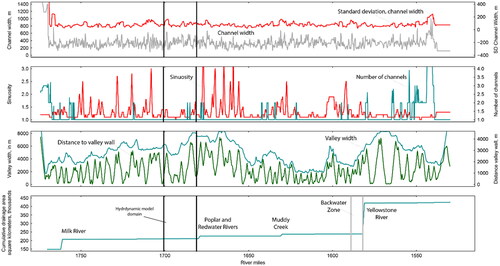
Results

Of the geomorphic variables, sinuosity, number of channels, valley width, and distance to the valley wall show considerable longitudinal variation (Figure A1). Table A1 shows summary statistics for the entire UPMOR segment, the model domain, and the upper and lower reaches within the model domain. The model domain has representative ranges of channel widths and standard deviation of channel widths; it has somewhat larger valley width but a representative range of distance from the channel to valley width; it has reaches with single-thread and multiple thread channels; the range of channel sinuosity (1–1.6) is less than some reaches that can range up to 4.9.

Part of the hydrodynamic and particle tracking analysis relies on comparison between contrasting upper and lower sections. The lower section is notable for having somewhat higher bankfull channel width and higher sinuosity (Table A1). Because the bankfull measures of channel complexity seemed to underestimate field-observable characteristics, we also count the number of channels evident during low-flow conditions as documented in the lowest modelled discharge. The average number of channels in the low-flow condition for the lower section is 2.3 while that for the upper section is 1.7 (Table A1).

The geomorphic classification indicates that the model domain captures a substantial amount of the geomorphic variation within Fort Peck – Lake Sakakawea segment of the UPMOR. Although the model domain lacks some of the more sinuous reaches, we believe that it captures many of the geomorphic features that are associated with hydraulic complexity and dispersal processes.

Appendix B.

Velocity validation and lateral eddy viscosity sensitivity

Appendix B consists of velocity cross sections used in model validation, detailed breakthrough curves, and transport metrics compared by lateral eddy viscosity (LEV) values.

Velocity cross sections

Figure B1.1. Comparisons of measured (red) and modelled (blue and black) depth-averaged velocities and depths for measurements made at cross-section 1 on June 10, 2018 (a and b, respectively), and July 1, 2019 (c and d, respectively). Solid blue lines represent values using hydrodynamics generated using the calibrated roughness parameter while the dashed black line represent hydrodynamics generated using the roughness parameter derived using Eq. (10)(10) $$\mathit{\text{Cd}}=\frac{n^{2}g}{h^{\raisebox{1ex}{$1$}\!\left/ \!\raisebox{-1ex}{$3$}\right.}}$$(10) .

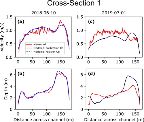
Figure B1.2. Comparisons of measured (red) and modelled (blue and black) depth-averaged velocities and depths for measurements made at cross-section 4 on June 10, 2018 (a and b, respectively), and September 9, 2018 (c and d, respectively). Solid blue lines represent values using hydrodynamics generated using the calibrated roughness parameter while the dashed black line represent hydrodynamics generated using the roughness parameter derived using Eq. (10)(10) $$\mathit{\text{Cd}}=\frac{n^{2}g}{h^{\raisebox{1ex}{$1$}\!\left/ \!\raisebox{-1ex}{$3$}\right.}}$$(10) .

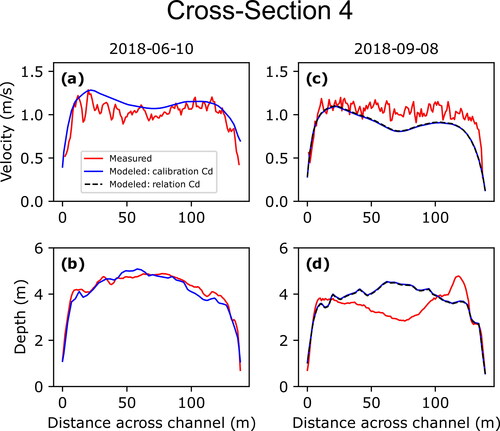
Figure B1.3. Comparisons of measured (red) and modelled (blue and black) depth-averaged velocities and depths for measurements made on June 10, 2018 (a and b, respectively), and September 8, 2018 (c and d, respectively) at cross-section 5. Solid blue lines represent values using hydrodynamics generated using the calibrated roughness parameter while the dashed black line represent hydrodynamics generated using the roughness parameter derived using Eq. (10)(10) $$\mathit{\text{Cd}}=\frac{n^{2}g}{h^{\raisebox{1ex}{$1$}\!\left/ \!\raisebox{-1ex}{$3$}\right.}}$$(10) .

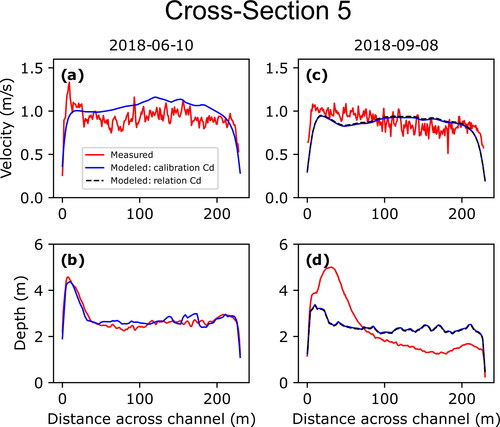
Breakthrough curves by LEV values

Figure B1.4. Comparisons of breakthrough curves from the 1-dimensional (1D) model, Lagrangian particle tracking (LPT) simulations, and larval catch field data for 1-day-post-hatch (DPH) larvae at stations 1 and 2 for LEVx0.5 (a and b, respectively), LEVx1 (c and d, respectively), and LEVx2 (e and f, respectively).

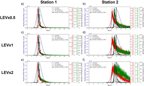
Figure B1.5. Comparisons of breakthrough curves from the 1-dimensional (1D) model, Lagrangian particle tracking (LPT) simulations, and larval catch field data for 5-days-post-hatch (DPH) larvae at stations 1 and 2 for LEVx0.5 (a and b, respectively), LEVx1 (c and d, respectively), and LEVx2 (e and f, respectively).

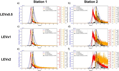
Transport metrics by LEV values

Figure B1.6. Comparison of percent particles retained for the upper reach (red) and lower reach (blue) for passive (first column), active75pct (second column), and active50pct (third column) vertical movement scenarios for LEVx0.5 (a, b, and c, respectively), LEVx1 (d, e, and f, respectively), and LEVx2 (g, h, and i, respectively).

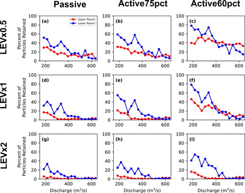
Figure B1.7. Comparison of mean residence time for the upper reach (red) and lower reach (blue) for passive (first column), active75pct (second column), and active50pct (third column) vertical movement scenarios for LEVx0.5 (a, b, and c, respectively), LEVx1 (d, e, and f, respectively), and LEVx2 (g, h, and i, respectively).

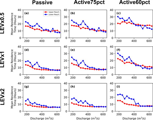
Figure B1.8. Comparison of mean transit time for the upper reach (red) and lower reach (blue) for passive (first column), active75pct (second column), and active50pct (third column) vertical movement scenarios for LEVx0.5 (a, b, and c, respectively), LEVx1 (d, e, and f, respectively), and LEVx2 (g, h, and i, respectively).

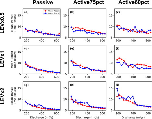
Table A1. Medians of geomorphic variables for the upper Missouri River, model domain, and upper and lower subsections.

	n	Average bankfull channel width, m	Standard deviation of channel width, m	Average channel sinuosity @ 3200 m	Maximum channel sinuosity @ 3200 m	Bankfull number of channels	Low-flow number of channels	Average valley width, m	Distance, channel to valley, m
Fort Peck Segment	2,448	323.0	105.8	1.25	4.91	1.17	NA	5,067	1,313
Model domain	224	359.3	106.1	1.15	1.58	1.02	2.0	6,237	1,380
Upper section	112	345.9	113.6	1.12	1.58	1.00	1.7	5,198	968
Lower section	112	369.9	100.2	1.18	1.47	1.04	2.3	7,054	1,703

Data are tabulated by 160 m sub reaches. Data source: Jacobson et al. (2023a). [NA, not applicable.].

References

- Braaten P, Fuller D, Lott R, Ruggles M, Brandt T, Legare R, Holm R. 2012. An experimental test and models of drift and dispersal processes of pallid sturgeon (Scaphirhynchus albus) free embryos in the Missouri River. Environ Biol Fish. 93(3):377–392. doi: 10.1007/s10641-011-9925-9.
- Braaten PJ, Campana SE, Fuller DB, Lott RD, Bruch RM, Jordan GR. 2015. Age estimations of wild pallid sturgeon (Scaphirhynchus albus, Forbes & Richardson 1905) based on pectoral fin spines, otoliths and bomb radiocarbon: inferences on recruitment in the dam-fragmented Missouri River. J Appl Ichthyol. 31(5):821–829. doi: 10.1111/jai.12873.
- Braaten PJ, Fuller DB, Holte LD, Lott RD, Viste W, Brandt TF, Legare RG. 2008. Drift dynamics of larval pallid sturgeon and shovelnose sturgeon in a natural side channel of the Upper Missouri River, Montana. N American J Fish Manag. 28(3):808–826. doi: 10.1577/M06-285.1.
- Braaten PJ, Fuller DB, Lott RD, Ruggles MP, Holm RJ. 2010. Spatial distribution of drifting pallid sturgeon larvae in the Missouri River inferred from two net designs and multiple sampling locations. N American J Fish Manag. 30(4):1062–1074. doi: 10.1577/M09-149.1.
- Braaten PJ, Holley C. 2021. Pallid sturgeon free embryo drift and dispersal experiment data from the Upper Missouri River, Montana and North Dakota, 2019: U.S. Geological Survey Data Release. doi: 10.5066/P9N2MFV8.
- Braaten PJ, Holm RJ, Powell J, Heist EJ, Buhman AC, Holley CT, Delonay AJ, Haddix TM, Wilson RH, Jacobson RB. 2022. Growth and survival rates of dispersing free embryos and settled larvae of pallid sturgeon (Scaphirhynchus albus) in the Missouri River, Montana and North Dakota. Environ Biol Fish. 105(8):993–1014. doi: 10.1007/s10641-022-01294-w.
- Call BC, Erwin SO, Bulliner EA. 2024. Supporting files for particle tracking simulations of the Upper Missouri River near Wolf Point, MT. U.S. Geological Survey data. doi: 10.5066/P975PH68.
- Chojnacki KA, Dodson MJ, George AE, Candrl JS, Delonay AJ. 2022. Ontogenetic development of pallid sturgeon (Scaphirhynchus albus) and shovelnose sturgeon (Scaphirhynchus platorynchus) from hatch through yolk absorption. Ecol Freshwater Fish. 32(1):209–231. doi: 10.1111/eff.12680.
- Chojnacki KA, Erwin SO, George AE, Candrl JS, Jacobson RB, Delonay AJ. 2020. Physical characteristics and simulated transport of pallid sturgeon and shovelnose sturgeon eggs. J Freshwater Ecol. 35(1):73–94. doi: 10.1080/02705060.2020.1736191.
- Coutant CC. 2004. A riparian habitat hypothesis for successful reproduction of white sturgeon. Rev Fish Sci. 12(1):23–73. (doi: 10.1080/10641260490273023.
- Delonay AJ, Chojnacki KA, Jacobson RB, Albers JL, Braaten PJ, Bulliner EA, Elliott CM, Erwin SO, Fuller DB, Haas JD, et al. 2016. Ecological requirements for pallid sturgeon reproduction and recruitment in the Missouri River: a synthesis of science, 2005-2012. U.S. Geological Survey Scientific Investigations Report 2015–5145. 224. doi: 10.3133/sir20155145.
- Elliott CM, Delonay AJ, Chojnacki KA, Jacobson RB. 2020. Characterization of Pallid Sturgeon (Scaphirhynchus albus) spawning habitat in the Lower Missouri River. J Appl Ichthyol. 36(1):25–38. doi: 10.1111/jai.13994.
- Erwin SO, Bulliner EA, Fischenich C, Jacobson RB, Braaten PJ, Delonay AJ. 2018. Evaluating flow management as a strategy to recover an endangered sturgeon species in the Upper Missouri River, USA. River Res Apps. 34(10):1254–1266. doi: 10.1002/rra.3371.
- Erwin SO, Jacobson RB. 2014. Influence of channel morphology and flow regime on larval drift of pallid sturgeon on the Lower Missouri River. River Res Apps. 31(5):538–551. doi: 10.1002/rra.2752.
- Fischenich JC, Mccomas R, Meier D, Tripe J, Pridal D, Boyd P, Gibson S, Hickey J, Econopouly T, Strong L. 2018. Habitat analyses for the Missouri River effects analysis. 176 pages. https://usace.contentdm.oclc.org/utils/getfile/collection/p16021coll7/id/8074.
- Fischenich JC, Reynolds SA, Halteman P. 2021. Fort Peck EIS Alternative effects on pallid sturgeon: Model documentation and study report. 280 pages. https://usace.contentdm.oclc.org/utils/getfile/collection/p16021coll7/id/8074.
- Fischer HB, List EJ, Koh RCY, Imberger J, Brooks NH. 1979. Mixing in Inland and Coastal Waters. New York (NY): Academic.
- Fischer HB. 1973. Longitudinal dispersion and turbulent mixing in open channel flow. Annu Rev Fluid Mech. 5(1):59–78. doi: 10.1146/annurev.fl.05.010173.000423.
- Galat DL, Berry CR, Jr., Peters EJ, White RG. 2005. Missouri River Basin. In: Benke AC, Cushing CE, editors. Rivers of North America. Oxford: Elsevier.
- Garcia T, Jackson PR, Murphy EA, Valocchi AJ, Garcia MH. 2013. Development of a Fluvial Egg Drift Simulator to evaluate the transport and dispersion of Asian carp eggs in rivers. Ecol Modell. 263:211–222. doi: 10.1016/j.ecolmodel.2013.05.005.
- Garcia T, Murphy EA, Jackson PR, Garcia MH. 2015. Application of the FluEgg model to predict transport of Asian carp eggs in the Saint Joseph River (Great Lakes tributary). J Great Lakes Res. 41(2):374–386. doi: 10.1016/j.jglr.2015.02.003.
- Guy CS, Treanor HB, Kappenman KM, Scholl EA, Ilgen JE, Webb M. 2015. Broadening the regulated-river management paradigm: a case study of the forgotten dead zone hindering pallid sturgeon recovery. Fisheries. 40(1):6–14. doi: 10.1080/03632415.2014.987236.
- Humphries P, King A, Mccasker N, Kopf RK, Stoffels R, Zampatti B, Price A. 2019. Riverscape recruitment: a conceptual synthesis of drivers of fish recruitment in rivers. Can J Fish Aquat Sci. 77(2):213–225. doi: 10.1139/cjfas-2018-0138.
- Jacobson RB, Elliott CM, Bulliner EA. 2023a. Geomorphic classification framework for assessing reproductive ecology of Scaphirhynchus albus (pallid sturgeon), Fort Peck segment, Upper Missouri River, Montana and North Dakota. Scientific Investigations Report 2023-5109. 15 pages. doi: 10.3133/sir20235109.
- Jacobson RB, Elliott CM, Bulliner EA. 2023b. Geomorphic variables for classification of the Upper Missouri River, Montana and North Dakota. U.S. Geological Survey data. doi: 10.5066/P92HVKT3.
- Jacobson RB, Elliott CM, Huhmann BL. 2010. Development of a channel classification to evaluate potential for cottonwood restoration, lower segments of the Middle Missouri River, South Dakota and Nebraska. Scientific Investigations Report 2010-5208. Scientific Investigations Report 2010-5208. 38 pages. doi: 10.3133/sir20105208.
- Jordan GR, Heist EJ, Braaten PJ, Delonay AJ, Hartfield P, Herzog DP, Kappenman KM, Webb M. 2016. Status of knowledge of the pallid sturgeon (Scaphirhynchus albus Forbes and Richardson, 1905). J Appl Ichthyol. 32(Suppl. S1):191–207. doi: 10.1111/jai.13239.
- Kynard B, Henyey E, Horgan M. 2002. Ontogenetic behaviour, migration, and social behaviour of pallid sturgeon (Scaphirhynchus albus) and shovelnose sturgeon (S. platorynchus) with notes on the adaptive significance of body color. Environ Biol Fish. 63(4):389–403. doi: 10.1023/A:1014950202783.
- Lechner A, Keckeis H, Humphries P. 2016. Patterns and processes in the drift of early developmental stages of fish in rivers: a review. Rev Fish Biol Fisheries. 26(3):471–489. doi: 10.1007/s11160-016-9437-y.
- Lechner A, Keckeis H, Schludermann E, Humphries P, Mccasker N, Tritthart M. 2014. Hydraulic forces impact larval fish drift in the free flowing section of a large European river. Ecohydrology. 7(2):648–658. doi: 10.1002/eco.1386.
- Li G, Elliott CM, Call BC, Chapman DC, Jacobson RB, Wang B. 2023. Evaluations of Lagrangian egg drift models: from a laboratory flume to large channelized rivers. Ecol Modell. 475:110200. doi: 10.1016/j.ecolmodel.2022.110200.
- Li G, Wang B, Elliott CM, Call BC, Chapman DC, Jacobson RB. 2022. A three-dimensional Lagrangian particle tracking model for predicting transport of eggs of rheophilic-spawning carps in turbulent rivers. Ecol Modell. 470:110035. doi: 10.1016/j.ecolmodel.2022.110035.
- Marotz BL, Lorang MS. 2018. Pallid sturgeon larvae: the drift dispersion hypothesis. J Appl Ichthyol. 34(2):373–381. doi: 10.1111/jai.13569.
- Mccasker N, Humphries P, Meredith S, Klomp N. 2014. Contrasting patterns of larval mortality in two sympatric riverine fish species: a test of the critical period hypothesis. PLoS One. 9(10):e109317. doi: 10.1371/journal.pone.0109317.
- Mcdonald R, Nelson JM. 2020. A Lagrangian particle-tracking approach to modelling larval drift in rivers. J Ecohydraul. 6(1):17–35. doi: 10.1080/24705357.2019.1709102.
- Mcdonald RR, Prescott AB, Foks NL. 2020. fluvial-particle. doi: 10.5066/P9K1U4O0.
- Mion JB, Stein RA, Marschall EA. 1998. River discharge drives survival of larval walleye. Ecol Appl. 8(1):88–103. doi: 10.1890/1051-0761(1998)008[0088:RDDSOL]2.0.CO;2.
- Mrnak J. 2019. Effect of water velocity and temperature on energy use, behavior, and mortality of pallid sturgeon Scaphirhynchus albus larvae. Master of Science in Wildlife and Fisheries Sciences, South Dakota State University. https://openprairie.sdstate.edu/cgi/viewcontent.cgi?article=4296&context=etd.
- Mrnak JT, Heironimus LB, James DA, Chipps SR. 2020. Effect of water velocity and temperature on energy use, behaviour and mortality of pallid sturgeon Scaphirhynchus albus larvae. J Fish Biol. 97(6):1690–1700. doi: 10.1111/jfb.14532.
- Nelson JM, Mcdonald RR. 1997. Mechanics and modeling of flow and bed evolution in lateral separation eddies. Glen Canyon Environmental Studies Report. 68 pages. http://www.riversimulator.org/Resources/GCMRC/PhysicalResources/Nelson1996.pdf.
- Nelson JM, Shimizu Y, Abe T, Asahi K, Gamou M, Inoue T, Iwasaki T, Kakinuma T, Kawamura K, Kimura I, et al. 2016. The international river interface cooperative: public domain flow and morphodynamics software for education and applications. Adv Water Resour. 93(July 2016):62–74. doi: 10.1016/j.advwatres.2015.09.017.
- Parsons DR, Jackson PR, Czuba JA, Engel FL, Rhoads BL, Oberg KA, Best JL, Mueller DS, Johnson KK, Riley JD. 2013. Velocity Mapping Toolbox (VMT): a processing and visualization suite for moving-vessel ADCP measurements. Earth Surf Processes Landf. 38(11):1244–1260. doi: 10.1002/esp.3367.
- Python Core Team. 2018. Python: A dynamic, open source programming language. 3.6.5 ed. Beaverton (OR): Python Software Foundation.
- U.S. Army Corps of Engineers. 2015. Missouri River Recovery Program Managment Plan Environmental Impact Statement Existing Conditions Unsteady HEC-RAS Model Calibration Report. 598 pages. https://usace.contentdm.oclc.org/digital/collection/p16021coll7/id/3067/.
- U.S. Army Corps of Engineers. 2021. Fort Peck Dam Test Release Final Environmental Impact Statement. 608 pages. https://usace.contentdm.oclc.org/digital/collection/p16021coll7/id/19203/rec/76.
- U.S. Geological Survey. 2021. USGS ImageryOnly Base Map. https://apps.nationalmap.gov/services/.
- U.S. Geological Survey. 2022. National Water Information System data available on the World Wide Web (USGS Water Data for the Nation). doi: 10.5066/F7P55KJN.
- United States Department of Agriculture. 2019. National Agricultural Imagery Program. doi: 10.5066/F7QN651G.