Normalized coefficients of prediction accuracy for comparative forecast verification and modeling

Abstract

The error coefficients $\text{MSE}$, $\text{RMSE},\text{ MAE}$, and the linear model measures r and R² are used in several disciplines to quantify the agreement between predicted and observed numerical data. Typical applications include forecast verification and model calibration. However, these coefficients have major drawbacks: Whereas the error coefficients are not comparable between data with different scaling, the measures from linear models are insensitive to additive or multiplicative biases. Here, we present a new categorization of the various normalizations and other modifications proposed in the literature to overcome these problems. We then propose a novel and simple idea to normalize $\text{MSE},\text{ RMSE}$, and $\text{MAE}$ in analogy to the construction of r: We divide each error coefficient by its maximum that is possible when considering the given sets of predictions and observations separately. Unlike existing normalizations of error coefficients or skill scores, our new normalized coefficients treat observations and predictions symmetrically and do not rely on past data. As a result, they are not subject to artificial bias or spurious accuracy due to a long-term trend in the data. After discussing properties of the new coefficients and illustrating them with simple artificial data, we demonstrate their advantages with real data from atmospheric science.

Keywords:

• Forecast evaluation
• model calibration
• normalized RMSE, MAE
• point forecast

1 Introduction

Every prediction has to stand the test of observation. The most familiar everyday example is probably the weather forecast. The World Meteorological Organization (WMO 2019) states that for each station, forecasts of certain weather parameters, such as temperature, should be verified against the observed parameter by calculating the mean error, the mean absolute error ($\text{MAE}$) and the root mean square error ($\text{RMSE}$) over the days of a month; for the formulae, see Table 1. However, the WMO (2019, 99) does not recommend calculating such error coefficients to verify precipitation forecasts, probably for the following reason: Imagine a precipitation forecast with a $\text{MAE}$ of 5 mm at one station and another with a $\text{MAE}$ of 50 mm at another station where it rains on average ten times as much. Which forecast would you call “more accurate”? In the present paper we call this kind of problem comparative forecast verification. A related problem is the calibration of models to observations obtained under different conditions. In the example above, consider a (fictitious) weather model with one or more free parameters that are to be determined in such a way that, over a series of days and over the two stations, the precipitation predicted by the model deviates “as little as possible” from the observed precipitation. If the fit criterion to be minimized depends on the absolute values, such as the MAE, then the station with the higher level of precipitation will exert a greater influence on the result. We call this type of problem comparative modeling. It should be noted that in forecast verification, the observations used to evaluate the predictions are made later in time, whereas in modeling, the observations are made first and the predictions are based on them.

Table 1 Formulae and bounds of five widely used classical coefficients of prediction accuracy. $x_1,\dots ,x_n$ are the predicted values, $y_1,\dots ,y_n$ the corresponding observed values. The difference $d_i=y_i-x_i$ is the prediction error for the ith data point. For more notations and relationships, see the text and the Glossary in Supplementary Section A.

Name	Formulae	Eq.	Bounds
Mean Absolute Error	$\text{MAE}=\frac{1}{n}{\sum }_{i=1}^n|y_i-x_i|=\frac{1}{n}{\sum }_{i=1}^n\left|d_i\right|$.	(1)	$0\le \text{MAE}$
Mean Squared Error	$\text{MSE}=\frac{1}{n}{\sum }_{i=1}^n{(y_i-x_i)}^2=\frac{1}{n}{\sum }_{i=1}^n{d}_i{}^2$.	(2)	$0\le \text{MSE}$
Root Mean Squared Error	$\text{RMSE}=\sqrt{\text{MSE}}$.	(3)	$0\le \text{RMSE}$
Linear correlation (Pearson’s product-moment correlation)	$r=\frac{S_{\mathit{\text{xy}}}}{S_x S_y}=b\frac{S_x}{S_y}$.	(4)	$-1\le r\le 1$
Proportion of explained variance (determination coefficient of regression)	$R^2=\frac{S_{\widehat{y}}^2}{S_y^2}=r^2$.	(5)	$0\le R^2\le 1$

A variety of disciplines face the problem of quantifying the agreement between predicted and observed data (see e.g. the overview of forecast papers from several disciplines in Gneiting 2011, Table 2). As well as in the atmospheric sciences like meteorology, climatology, and hydrology, forecast verification and modeling play a crucial role in economics (quantities of demand, production, sales, consumption, profit and loss are being modeled and forecast, but also less predictable quantities such as exchange rates or stock prices, see e.g. the textbook by Hyndman and Athanasopoulos 2021), in the life sciences (population dynamics, quantitative genetics, agriculture, see e.g. Istas 2005), and even in cognitive psychology (reaction times, error rates, eye movement parameters, e.g. Engbert et al. 2005; Müller-Plath and Pollmann 2003; Van Zandt and Townsend 2012). In each of these disciplines, the researcher may face a situation where datasets with different scales need to be handled simultaneously. i.e. comparative forecast verification and modeling.

Table 2 Data situations where the common coefficients from Table 1 are suitable (normal text) or not (indicated by $\neg \{\dots \}$); LM = linear model; the scope for our new coefficients are the situations where none of the common coefficients are suitable, i.e. the framed leftmost and rightmost cells in the bottom row.

	“Forecast verification”	“Modelling”
	Predictions made before observations	Predictions made from observations
Data set(s)	by any means (LM or other)	by a LM	other than by a LM
Uniform scaling	MAE, MSE/RMSE	MAE, MSE/RMSE	MAE, MSE/RMSE
	$\neg \{r,R^2\}$	r, R^2	$\neg \{r,R^2\}$
Different scaling (“Comparative”)	$\begin{array}{c}\neg \left\{\text{MAE, MSE/RMSE}\right\}\\ \neg \{r,R^2\}\end{array}$	$\neg \left\{\text{MAE, MSE/RMSE}\right\}$ r, R^2	$\begin{array}{c}\neg \left\{\text{MAE, MSE/RMSE}\right\}\\ \neg \{r,R^2\}\end{array}$

The classical coefficients widely used to quantify the agreement between predicted and observed numerical data are not suitable for the above situations: Whereas the error coefficients such as the $\text{RMSE}$ and the $\text{MAE}$ are not comparable between data with different scaling, measures from linear models such as the correlation r and the determination coefficient R² are insensitive to additive or multiplicative biases (see below). To overcome these problems, different disciplines have produced various normalizations and other modifications of the above coefficients, each of which has its own advantages and areas of application, but in turn has introduced new problems in other areas. In this paper, we first propose a novel scheme for categorizing the numerous modified coefficients in order to systematize and guide interdisciplinary discussions on their advantages and disadvantages in different application areas. Then we propose a new and simple idea for normalizing the classical error coefficients that is suitable for “comparative forecast verification” and “comparative modeling.” It is restricted to univariate numerical variables in a finite sample, called deterministic or point forecast in some disciplines. A classic example is a time series as found in atmospheric sciences or economics. Problems of inferential statistics are not covered.

Let us start with some comments on terminology: Depending on the discipline, a coefficient that compares predictions to observations is termed fit error, accuracy, association, skill, etc. In atmospheric sciences, coefficients that measure the correspondence in absolute values (as in the above examples) are referred to as accuracy, whereas coefficients that measure it relative to that of a reference forecast are termed skill (Potts 2012). Disciplines that are more concerned with model fitting than with forecasting often summarize all such coefficients as goodness-of-fit measures, whether they are in absolute values or not, and use a variety of terms in detail. In this paper, we will refer to any coefficient reflecting the degree of correspondence between predicted and observed data as prediction accuracy, regardless of its sign, normalization, or whether it’s relative to a reference or not.

1.1 Common coefficients of prediction accuracy

The basis for quantifying prediction accuracy is the joint (bivariate) distribution of predicted values $x_1,\dots ,x_n$, obtained by any means, and the corresponding observed values $y_1,\dots ,y_n$ in a finite sample of numerical data (notation from Gneiting 2011). Figure 1 shows some sample data. In forecast verification, where the observations are used to evaluate the predictions, it seems more intuitive to denote the data pairs by (x_i, y_i) and to plot the predictions on the abscissa and the observations on the ordinate of the coordinate system (see e.g. Wilks 2019, 370 and Fig. 9.8). In modeling, where the observations are used to estimate parameters of a model (model calibration), it seems more intuitive to denote the data pairs by (y_i, x_i) and to plot the observations on the abscissa and the predictions on the ordinate of the coordinate system. In this cross-application and cross-disciplinary work, we need an abstract representation and have chosen the first. It can be converted to the second at any point.

Fig. 1 Comparison of predictions and observations in a finite sample of n cases in a “time series format” (upper panel; with an order on the pairs of data) and a scatterplot format of the bivariate distribution (lower panel). The predicted values are denoted with $x_1,\dots ,x_n$, and the corresponding observed values with $y_1,\dots ,y_n$. Since the accuracy coefficients do not rely on the order of the sample points, the lower panel forms the starting point of the present paper. The solid diagonal shows perfect prediction (all y_i = x_i). The dashed line is the regression line of observations on predictions ${\widehat{y}}_i=a+b x_i$ (drawn to illustrate the difference between high correlation and good prediction).

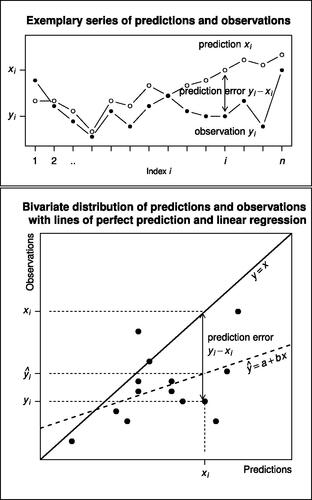
The index $i=1,\dots ,n$ may represent points in time (e.g. years in economy), points in space (e.g. grid points in meteorology), experimental trials (in cognitive psychology), and so on. Whether the order $1,\dots n$ is meaningful (which we call “time series format”) or not, depends on the application area. For the prediction accuracy coefficients developed here, it is not meaningful.

The difference $d_i=y_i-x_i$ is the prediction error for the ith data point. Throughout the paper we assume that the variances of the predictions and observations $S_x^2,S_y^2>0$, i.e. that neither of the two data series is constant. The prediction is perfect if all the observed values are equal to the predicted values (i.e. lie on the diagonal in the scatterplot in Figure 1). It gets worse as the agreement decreases, and is worthless if the relationship between observations and predictions is inverse. To illustrate the problem of the correlation coefficient r as a measure of prediction accuracy and its square R², which are both concepts within the framework of linear least squares regression, we contrast the line of perfect prediction y_i = x_i with the line ${\widehat{y}}_i=a+b x_i$ of the linear regression of the observations $y_1,\dots ,y_n$ on the predictions $x_1,\dots ,x_n$. Notations and relationships are given in more detail in the Glossary in Supplementary Section A.

Table 1 shows the five widely used coefficients of prediction accuracy mentioned above. As they are well known and found in any textbook, no specific references are given. To visualize each concept, the reader can use Figure 1.

Coefficients of the first type are the error coefficients $\text{MAE},\text{ MSE}$ and $\text{RMSE}$ (eqs. (1)–(3) in Table 1). In order to remove the units of measurement from the coefficients, the various disciplines have developed various normalizations and modifications of the error coefficients (see the literature review in Section 2 and Table 3).

Table 3 Examples of the four types of transformations to de-scale and de-bias the coefficients from Table 1.

Type	Original coefficient	Modified coefficient (examples in literature)	Alternatives (coefficient names from the respective literature) and remarks
A.1	$\text{MSE}$	$\text{NMSE}=\frac{\text{MSE}}{S_y^2}$ (Pokhrel and Gupta 2010, hydrology; Engbert et al. 2005, psychology; Hammi and Miftah 2015, engineering)	NMSE’ (Gupta and Kling 2011, hydrology); NNSE (Nossent and Bauwens 2012, hydrology); NSE (Nash and Sutcliffe 1970, hydrology); ${\text{NSE}}_{\text{cor}}$, KGE (Gupta et al. 2009, hydrology); d, ${\mathrm{d}}_2$ (Willmott 1981, geosciences).
A.1	$\text{RMSE}$	$\text{NRMSE}=\frac{\text{RMSE}}{\overline{y}}$ (Otto 2019, Zambresky 1989, marine sciences)	Other NRMSE’s: divide $\text{RMSE}$ by $y_{\mathrm{\text{max}}}-y_{\mathrm{\text{min}}}$, Sy, or ${\text{IQR}}_y$ (Otto 2019, marine sciences; Jacobs and Ferris 2015, rehabilitation); NRMS (Stephen and Kazemi 2014, geology).
A.1	$\text{MAE}$	$\text{NMAE}=\frac{\text{MAE}}{y_{\mathrm{\text{max}}}-y_{\mathrm{\text{min}}}}$ (Goldberg et al. 2001, information sciences; Cantelmo et al. 2020, economics)	Other NMAE’s: divide $\text{MAE}$ by $\overline{y}$ or ymax (Abe et al. 2020, solar physics; Previsic et al. 2021, oceanography); ${\mathrm{E}}_1$ (Legates and McCabe 1999, hydrology); ${\mathrm{E}}_{\text{NMAE}},\mathrm{E}{\prime }_{\text{NMAE}}$ (Gustafson and Yu 2012, meteorology); ${\mathrm{d}}_1$ (Willmott et al. 1985, geosciences); $\text{MASE}$ (Hyndman and Koehler 2006, economics).
A.2	$\text{MSE}$	$\text{MSESS}=1-\frac{\text{MSE}}{{\text{MSE}}_{\text{ref}}}$ with ${\text{MSE}}_{\text{ref}}=\frac{1}{n}{\sum }_{i=1}^n{(y_i-{\overline{y}}_{\text{ref}})}^2$ and ${\overline{y}}_{\text{ref}}$ the mean value of a reference set of observations (Dequé 2012, p. 83, atmospheric sciences; Campbell and Thompson 2008, economics).	This skill score is interpreted as proportional improvement over the reference, in climatology usually a reference period agreed upon. Alternative names: ${\text{SS}}_{\text{clim}}$ (Wilks 2019, pp. 397, atmospheric sciences), $R_{\text{OS}}^2$ (Audrino et al. 2020, economics).
A.2	$\text{MAE}$	$\text{MAESS}=1-\frac{\text{MAE}}{{\text{MAE}}_{\text{ref}}}$.	Analogous to $\text{MSESS}$, same literature.
B.1	$\text{MAE}$	$\text{MAPE}=\frac{1}{n}{\sum }_{i=1}^n\left|\frac{y_i-x_i}{y_i}\right|·100$ (with or without factor 100; Armstrong and Collopy 1992, economics; Daum and Hecht 2009, psychology, called REE there.)	$\text{sMAPE}$ (Makridakis and Hibon 2000); $\text{MdRAE}$ (Armstrong and Collopy 1992), both economics; $\text{APE},\text{ RE}$ (Gneiting 2011, general).
B.2	r	$\text{ACC}=r_{x\prime y\prime }$ with $x{\prime }_i=x_i-y_{\text{ref},i}$ and $y{\prime }_i=y_i-y_{\text{ref},i}$ where $y_{\text{ref},i}=\frac{1}{m}{\sum }_{j=1}^m{y}_{j,i}$ is a climatological average at spatial point i, and $y_{j,i}$ the observed value at time step j at spatial point i. (Wilks 2019, p. 453; WMO, World Meteorological Organization 2023, atmospheric sciences)	“Anomaly correlation” The summation index i refers to a spatial (grid) point. The prediction and the observation at every grid point i are transformed into an anomaly, i.e. the difference of the current value to a temporal average value calculated over a reference period agreed upon (with summation index j), before the correlation over the spatial series is calculated.
B.2	$\text{MSE}$	$\text{MSE}(\text{CVBC})=\frac{1}{n}{\sum }_{i=1}^n{(y_i-x{\prime }_i)}^2$ where $x{\prime }_i$ is the “cross-validated bias corrected” prediction, i.e. $x{\prime }_i=x_i-\text{est}({\mathrm{B}}_{\text{add}})$. The estimated bias $\text{est}({\mathrm{B}}_{\text{add}})=x_{\text{ref}}-y_{\text{ref}}$ is calculated from a reference sample of predictions and observations, either formerly obtained or by excluding each target year in the averaging (cross validation). (Dequé 2012, p. 81; Maraun and Widmann 2018, atmospheric sciences)	Analogous to the “cross-validated bias correction” for $\text{MAE}$, same literature.

Notations are adapted to this paper (see the Glossary in Supplementary Section A)

Coefficients of the second type, the linear correlation coefficient r and its square R² (eqs. (4)–(5) in Table 1), measure the progression similarity of predicted and observed data, as roughly shown in the upper panel of Figure 1, but not their numerical agreement. The linear correlation of predictions and observations is their covariance S_xy normalized by its maximum ($\left|S_{\mathit{\text{xy}}}\right|\le S_x S_y$ because of the Cauchy-Schwarz inequality). Note that the perfect positive linear relationship r = 1, indicating that all points lie on a linear regression line with positive slope, is only a necessary but not a sufficient condition for perfect prediction accuracy, since the latter requires that all data points lie on the special regression line y_i = x_i, i.e. the line with a = 0 and b = 1 (see the bottom panel in Figure 1). It’s thus clear that r and R² are insensitive to linear scaling (eq. (A.9) in Supplementary Section A) and thus to additive and multiplicative prediction biases. In modeling, such biases can occur if the predictions are made by fitting the observations to a model that is not a linear least squares regression. In forecast verification, where predictions are made in advance of the verifying observations, biases can occur regardless of the means by which they were obtained. Although the problem is well-known (for detailed critiques, see e.g. Li 2017, geosciences; Waldmann 2019, genetics; Dequé 2012, atmospheric sciences), r and R² have been proposed for forecast verification (e.g. Von Storch and Zwiers 2002, 396), and are widely used (see for example Krause et al. 2005, hydrology; Norman et al. 2016, cognitive psychology; Daetwyler et al. 2008, genetics). However, similar to the error coefficients, some disciplines have developed modifications of r to eliminate such biases, as outlined in Section 2 and Table 3.

1.2 Aim of the paper and outline

The typical applications for our new prediction accuracy coefficients are situations where the drawbacks of both types of classic coefficients coincide (the framed cells in Table 2): The error coefficients ($\text{MSE},\text{ RMSE},\text{ MAE}$) are meaningless when the data is composed of data sets with different scaling (denoted by $\neg$ in the bottom row of the table). The goodness-of-fit measures from linear least-squares modeling (r, R²) are prone to bias if either the predictions are made before the observations that are used for verification (denoted by $\neg$ in the leftmost column of the table), or if the predictions are made from the observations they are evaluated against with, but by a method other than linear least squares modeling (rightmost column of the table). The intersection of drawbacks results in two typical use cases, “comparative forecast verification” and “comparative modeling with other than linear least squares models.” Here, our new normalizations come into play. (Of course, they are also applicable in the other cases.)

In order to overcome the problems of incomparable scaling and/or bias, various normalizations and other modifications of the above coefficients have already been proposed in the literature. To our knowledge, there is as yet no normalization of the coefficients of prediction accuracy that treats the two data sets, predicted and observed, symmetrically, and that does not rely on past (reference) data. Both of these introduce new biases or artificial skill when it comes to comparative forecasting and modeling. The aim of the present paper is to fill this gap. To do this, we apply the idea that was behind the construction of r, where the unit-dependent covariance is divided by the maximum value it can attain when the association of the two data sets is disregarded and the two sets are considered separately. Analogously, here we normalize the error coefficients $\text{MSE},\text{ RMSE}$, and $\text{MAE}$ by dividing them by the maximum value that each coefficient can attain when the given sets of predictions and observations are considered separately. The resulting normalized coefficients $\text{MSE*},\text{RMSE*}$, and $\text{MAE*}$ thus range between 0 and 1 (note that the normalized covariance, the correlation r, ranges between–1 and 1 because the covariance can be negative).

In Section 2, we review ideas of normalization and de-biasing from different disciplines and briefly discuss some of their advantages and problems. In Section 3, we algebraically develop our new normalizations $\text{MSE*},\text{RMSE*}$, and $\text{MAE*}$ for comparative forecast verification and modeling. By linearly rescaling $\text{MSE*}$, we also obtain an alternative prediction accuracy coefficient $\text{PAC}$, which is identical to the correlation coefficient r in the special case of standard scores (z-scaled data; see the Glossary in Supplementary Section A). In Section 4, we derive properties of our new normalized coefficients for the general case and illustrate them with some characteristics of predicted and observed data. In this context, we discuss the problem of a priori rescaling the data when modeling data sets with different scaling. In the final Section 5, we apply the new normalized coefficients $\text{MSE*},\text{RMSE*}$, and $\text{MAE*}$ to real data from atmospheric sciences and show that they are obviously the best choice for comparative forecast verification and modeling.

2 Normalization and de-biasing: literature review and problems

Due to the aforementioned drawbacks of the classic coefficients of prediction accuracy from Table 1, a plethora of proposals for their modification have emerged, which differ somewhat between disciplines. Since it is beyond the scope of this paper to analyze and discuss their mathematical properties and relationships in detail, we will only give a brief overview of the main lines of development. A deeper statistical treatment of some of them can be found in Gneiting (2011).

Hyndman and Koehler (2006) have already provided a useful categorization and an in-depth discussion of many modern coefficients of prediction accuracy, but with a focus on applications in economics and thus without including the accuracy measures that are popular in atmospheric and cognitive sciences, such as the NMSE (Pokhrel and Gupta 2010; Engbert et al. 2005, see the first line of Table 3). We therefore propose an alternative scheme for categorizing coefficients that may systematize and guide a more interdisciplinary discussion of advantages and disadvantages in different application areas. It starts from the classical coefficients $\text{MSE},\text{ RMSE},\text{ MAE}$, r and R² listed in Table 1, and categorizes existing ideas for scaling or bias removal as follows:

1. Calculate the coefficient from the raw data and then transform the coefficient

• (A.1) using measures from the sample data

• (A.2) using measures from past data (‘reference measures’).

1. Transform each data or pair of data

• (B.1) using data from the sample

• (B.2) using reference data, usually from the past

and then calculate the coefficient.

Table 3 gives examples of each type and literature from different disciplines. As described in the cited literature, each coefficient has its own advantages in some applications and disadvantages in others. For comparative forecast verification and modeling, none of the existing coefficients is ideal, so despite the abundance of coefficients of prediction accuracy, there is still a need for new ones dedicated to this application. Some of the following drawbacks will be illustrated in the case study in Section 5.

Almost all so-called “normalized” error coefficients of type A.1 use only measures of the sample of observations (S_y, $\overline{y},y_{\mathrm{\text{max}}}-y_{\mathrm{\text{min}}}$ etc.) to eliminate the scale of the error. Characteristics and outliers in the observations thus have a disproportionate influence (Ehret and Zehe 2011). Even the $\text{NMSE}\prime$ (Gupta and Kling 2011), where $\text{MSE}$ is divided by $S_x S_y$, the resulting “normalized” coefficient is asymmetrically bounded between [0, +$\infty$[, making it subject to distortion and bias.

Modifying a coefficient with measures from past (reference) data, i.e. type A.2, is problematic when the current data have changed relative to the reference, as in the case of climate change. Fricker et al. (2013) discusses in detail how this can lead to a “spurious skill” of the forecast, which would mislead the verification of the forecast and affect the choice of parameters in comparative modeling.

On the other hand, calculating coefficients on relative instead of original data (types B) distorts the information in the data and is therefore also not suitable for comparative forecast verification and modeling. Moreover, most relative error coefficients of type B.1 suffer from the same problem as those of A.1. For example, Armstrong and Collopy (1992) $\text{MAPE}$ does not treat observations and predictions symmetrically so that positive and negative errors do not contribute equally, and some, like $\text{MAPE}$, are not even defined if one or more observations are zero. Type B.2 shares the problems of A.2 in that anomalies are biased by long-term changes in the reference value (Fricker et al. 2013). The technique of correcting the bias a posteriori, i.e. changing the predicted values using the observed values as in the cross-validated bias correction (last row in Table 3) has been shown to introduce new artificial biases (Maraun and Widmann 2018).

So, after having critiqued all the lines of development theoretically, what is the state of the art practically when it comes to comparative forecast verification and modeling? For comparative forecast verification, some recent papers have simply used a selection of coefficients in parallel without problematizing what would happen in case of disagreement (Audrino et al. 2020; Rahman et al. 2016; Afshar and Bigdeli 2011), whereas others (e.g. Magnusson et al. 2022) used only a few well-founded coefficients and discussed their results separately. Goelzer et al. (2018) used $\text{RMSE}$ to compare different modeling techniques for predicting ice cover in Greenland across geographically not fully overlapping datasets, i.e. for comparing forecast errors of presumably different scales. Interestingly, the authors problematize their use of $\text{RMSE}$ in this case and suggest “an alternative choice of metric” (Goelzer et al. 2018, 1441). The latter paper is among those cited in the introductory chapter of the latest IPCC report on methodology for evaluating models against observations (Chen et al. 2021, 225), and our present research can fill this gap.

Comparative modeling, our second concern, seems to have been carried out so far using one of the “normalized” error coefficients (e.g. the NMSE, see Table 3) or some self-made coefficient based on it but adapted to include metric and categorical data (Voudouri et al. 2021, for numerical weather models; Khain et al. 2015, for cloud models). The dependence of the NMSE on the variability of observations, especially outlier observations, has already been mentioned. Other disciplines have no better solutions: In economics, for example, Singular Spectrum Analysis (SSA) (Golyandina et al. 2001) is popular for model-free forecasting. In psychology, comparative modeling is still completely avoided by restricting model calibration to data sets that have been a priori made comparable in their scaling by the use of standardized experimental conditions (e.g. Engbert et al. 2005; Müller-Plath et al. 2010). A normalized coefficient of prediction accuracy for comparative modeling would open up great opportunities for the discipline by allowing models to be fitted post hoc to data, e.g. response times, from different experiments. In the atmospheric sciences, the problem of calibrating climate models to (past) data is a major issue, as data sets are often not comparable in scale. In the absence of a suitable coefficient, model tuning is either avoided or done manually, and the model fit is often checked by visual inspection (Mauritsen et al. 2012; Mauritsen and Roeckner 2020). Interestingly, Burrows et al. (2018) report the results of a broad community survey on the fidelity of climate models. Respondents cited a “lack of robust statistical metrics” as the biggest barrier to systematically quantifying model fidelity (p. 1110). (These latter papers are also cited in the introductory chapter of the latest IPCC report, Chen et al. 2021, 182, 218).

3 Approach: new normalizations of the Mean Squared Error, its root, and the Mean Absolute Error: $\text{MSE*},\text{RMSE*},\text{MAE*}$

In this section, we normalize $\text{MSE},\text{ RMSE},$ and $\text{MAE}$ at their maximum possible values, given the predicted and observed data. Our normaliztion thus belongs to category A.1 above, with both data sets, the predicted and observed, being considered symmetrically.

3.1 Developing $\text{MSE*}$ and $\text{RMSE*}$

As mentioned above, our idea for normalizing the $\text{MSE}$ is the same as in defining the correlation r as the normalized covariance (see eq. (4) in Table 1): Just as the covariance is divided by its maximum value $S_x S_y$, yielding a coefficient that indicates the linear relationship between two variables while ignoring their univariate characteristics, we want to divide $\text{MSE}$ by its maximum value that is possible when predicted and observed data are considered separately. We determine this maximum by decomposing $\text{MSE}$ into univariate measures of the two distributions and the correlation r with known limits. This decomposition of $\text{MSE}$ is easily obtained from the computational formula for the uncorrected sample variance (eq. (A.5) in Supplementary Section A), applied to the prediction error $d=y-x$. By rearranging the formula, writing out the variance of a difference of variables (eq. (A.7) in supplementary section A), and applying the definition of the correlation, eq. (2) in Table 1 becomes (6) $$\begin{array}{c}\text{MSE}=\overline{d^2}=\overline{d}{ }^2+S_d^2\\ ={(\overline{y}-\overline{x})}^2+S_{y-x}^2\\ ={(\overline{y}-\overline{x})}^2+S_x^2+S_y^2-2 S_x S_y r.\end{array}$$(6)

Equation (6)(6) $$\begin{array}{c}\text{MSE}=\overline{d^2}=\overline{d}{ }^2+S_d^2\\ ={(\overline{y}-\overline{x})}^2+S_{y-x}^2\\ ={(\overline{y}-\overline{x})}^2+S_x^2+S_y^2-2 S_x S_y r.\end{array}$$(6) has already been derived by Murphy (1988) and geometrically visualized by Taylor (2001), therein Figure 2; see also our Supplementary Section D. Given the means and variances of the two data sets, it is obvious from eq. (6)(6) $$\begin{array}{c}\text{MSE}=\overline{d^2}=\overline{d}{ }^2+S_d^2\\ ={(\overline{y}-\overline{x})}^2+S_{y-x}^2\\ ={(\overline{y}-\overline{x})}^2+S_x^2+S_y^2-2 S_x S_y r.\end{array}$$(6) that the $\text{MSE}$ attains its maximum if and only if r attains its minimum, i.e. r =–1. In this case, eq. (6)(6) $$\begin{array}{c}\text{MSE}=\overline{d^2}=\overline{d}{ }^2+S_d^2\\ ={(\overline{y}-\overline{x})}^2+S_{y-x}^2\\ ={(\overline{y}-\overline{x})}^2+S_x^2+S_y^2-2 S_x S_y r.\end{array}$$(6) reads (7) $$\begin{array}{c}{\text{MSE}}_{\mathrm{\text{max}}}={(\overline{y}-\overline{x})}^2+S_x^2+S_y^2+2 S_x S_y\\ ={(\overline{y}-\overline{x})}^2+{(S_x+S_y)}^2.\end{array}$$(7)

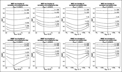
Fig. 2 $\text{MSE*}$ (top row) and $\text{RMSE*}$ (bottom row) as functions of correlation r and additive and multiplicative biases ${\mathrm{B}}_{\text{add}}$ and ${\mathrm{B}}_{\text{mult}}$. In order to depict the graphs independently of the scaling, the additive bias is given in units of the standard deviation of the predictions S_x (see eq. (12)(12) $$\text{MSE*}=1-2 \frac{{\mathrm{B}}_{\text{mult}} (1+r)}{{(\frac{{\mathrm{B}}_{\text{add}}}{S_x})}^2+{(1+{\mathrm{B}}_{\text{mult}})}^2}.$$(12) ).

By dividing the $\text{MSE}$ by its maximum, we arrive at our normalized mean squared error (8) $$\begin{array}{c}\text{MSE*}:=\frac{\text{MSE}}{{\text{MSE}}_{\mathrm{\text{max}}}}\\ =\frac{\frac{1}{n}\sum _{i=1}^n{(y_i-x_i)}^2}{{(\overline{y}-\overline{x})}^2+{(S_x+S_y)}^2}\\ =\frac{\overline{d^2}}{\overline{d}{ }^2+{(S_x+S_y)}^2}.\end{array}$$(8)

$\text{MSE*}$ is therefore the mean squared prediction error, divided by the sum of the squared mean prediction error and the squared sum of the standard deviations. By definition, it ranges between 0 and 1, with 0 denoting no error (perfect prediction) and 1 denoting the maximum error possible with the given means and standard deviations.

With the familiar rules of variance, covariance, and correlation, which are briefly summarized in the Glossary in Supplementary Section A, the $\text{MSE*}$ as defined in eq. (8)(8) $$\begin{array}{c}\text{MSE*}:=\frac{\text{MSE}}{{\text{MSE}}_{\mathrm{\text{max}}}}\\ =\frac{\frac{1}{n}\sum _{i=1}^n{(y_i-x_i)}^2}{{(\overline{y}-\overline{x})}^2+{(S_x+S_y)}^2}\\ =\frac{\overline{d^2}}{\overline{d}{ }^2+{(S_x+S_y)}^2}.\end{array}$$(8) can be reformulated in a couple of ways. The following reformulation may be useful for examining its properties: (9) $$\text{MSE*}=1-2 \frac{S_x S_y+S_{\mathit{\text{xy}}}}{(\overline{y}-\overline{x}){ }^2+{(S_x+S_y)}^2}.$$(9)

Another reformulation describes $\text{MSE*}$ as a function of correlation and biases. Let (10) $${\mathrm{B}}_{\text{add}}=\overline{d}=\overline{y}-\overline{x}.$$(10) denote the additive prediction bias, i.e. the mean prediction error and thereby the difference of means. Further, let (11) $${\mathrm{B}}_{\text{mult}}=\frac{S_y}{S_x}.$$(11) denote the multiplicative prediction bias as the ratio of dispersions (standard deviations) of observed and predicted values. Then, (12) $$\text{MSE*}=1-2 \frac{{\mathrm{B}}_{\text{mult}} (1+r)}{{(\frac{{\mathrm{B}}_{\text{add}}}{S_x})}^2+{(1+{\mathrm{B}}_{\text{mult}})}^2}.$$(12)

The proofs are in Supplementary Section B (eqs. (B.8), (B.9)) together with some further reformulations. We will call a prediction unbiased if it has neither an additive nor a multiplicative bias, i.e. if ${\mathrm{B}}_{\text{add}}=0$ and ${\mathrm{B}}_{\text{mult}}=1$. In this case, eq. (12)(12) $$\text{MSE*}=1-2 \frac{{\mathrm{B}}_{\text{mult}} (1+r)}{{(\frac{{\mathrm{B}}_{\text{add}}}{S_x})}^2+{(1+{\mathrm{B}}_{\text{mult}})}^2}.$$(12) implies (13) $$\text{MSE*}=\frac{1-r}{2}.$$(13)

The normalized root mean squared error is the square root of $\text{MSE*}$: (14) $$\text{RMSE*}:=\sqrt{\text{MSE*}}.$$(14)

$\text{RMSE*}$ also ranges between 0 and 1. Since $\text{MSE*}$ and $\text{RMSE*}$ are monotonically related, they can be used interchangeably in most applications, differing only in interpretation.

If one prefers a true “prediction accuracy coefficient” (PAC) that measures prediction accuracy with the same bounds as the correlation coefficient r measures linear relationship, one may want to linearly rescale the $\text{MSE*}$: (15) $$\text{PAC}:=1-2·\text{MSE*}.$$(15)

The $\text{PAC}$ ranges between–1 and 1. Prediction accuracy is low when $\text{PAC}\le 0$, and worst for $\text{PAC}=-1$. Positive values indicate increasingly better prediction accuracy, with $\text{PAC}=1$ being the best (every y_i = x_i). In the case of unbiased predictions, $\text{MSE*}=0.5 (1-r)$ and $\text{PAC}=r$, which is most easily seen from eq. (12)(12) $$\text{MSE*}=1-2 \frac{{\mathrm{B}}_{\text{mult}} (1+r)}{{(\frac{{\mathrm{B}}_{\text{add}}}{S_x})}^2+{(1+{\mathrm{B}}_{\text{mult}})}^2}.$$(12) .

3.2 Developing $\text{MAE*}$

For a coefficient that is robust against outliers, one might want to normalize the $\text{MAE}$ instead of the $\text{MSE}$. This is done analogously: We first determine the maximum value of the $\text{MAE}$ given the two univariate data sets and then divide the $\text{MAE}$ by its maximum.

Using the triangle inequality, the upper bound of each component of the $\text{MAE}$ is (16) $$\begin{array}{c}|y_i-x_i|=|(\overline{y}-\overline{x})-(x_i-\overline{x})+(y_i-\overline{y})|\\ \le |\overline{y}-\overline{x}|+|x_i-\overline{x}|+|y_i-\overline{y}|.\end{array}$$(16)

By summing up and dividing by n, the upper bound of the $\text{MAE}$ is thus (17) $${\text{MAE}}_{\mathrm{\text{max}}}=|\overline{y}-\overline{x}|+\text{MAD}(x)+\text{MAD}(y),$$(17) where $\text{MAD}(x)$ denotes the mean absolute deviation from the mean, an alternative measure of the spread of a data set (see the glossary in Supplementary Section A). By dividing the $\text{MAE}$ by this maximum, we arrive at our normalized mean absolute error (18) $$\begin{array}{c}\text{MAE*}:=\frac{\text{MAE}}{{\text{MAE}}_{\mathrm{\text{max}}}}\\ =\frac{\frac{1}{n}\sum _{i=1}^n|y_i-x_i|}{|\overline{y}-\overline{x}|+\text{MAD}(x)+\text{MAD}(y)}\\ =\frac{\overline{\left|d\right|}}{\left|\overline{d}\right|+|\text{MAD}(x)+\text{MAD}(y)|}.\end{array}$$(18)

$\text{MAE*}$ is thus the mean absolute prediction error, divided by the sum of the mean absolute prediction error and the sum of the spreads, expressed as mean absolute deviation. By definition, the coefficient $\text{MAE*}$ ranges between 0 and 1, with 0 denoting no error (perfect prediction) and 1 denoting maximum error. Note the structural similarity of $\text{MAE*}$ to $\text{MSE*}$ in eq. (8)(8) $$\begin{array}{c}\text{MSE*}:=\frac{\text{MSE}}{{\text{MSE}}_{\mathrm{\text{max}}}}\\ =\frac{\frac{1}{n}\sum _{i=1}^n{(y_i-x_i)}^2}{{(\overline{y}-\overline{x})}^2+{(S_x+S_y)}^2}\\ =\frac{\overline{d^2}}{\overline{d}{ }^2+{(S_x+S_y)}^2}.\end{array}$$(8) . The absolute value symbol around the sum of $\text{MAD}$s in the denominator of the last expression has been placed to emphasize this.

4 Properties of the new coefficients

In this section, we examine how $\text{MSE*},\text{RMSE*}$, and $\text{MAE*}$ behave in relation to characteristics of predicted and observed data. We start in Section 4.1 by drawing some graphs of $\text{MSE*}$ and $\text{RMSE*}$ as a function of the additive bias (difference of means), the multiplicative bias (ratio of standard deviations), and the correlation r between predictions and observations (Figure 2).

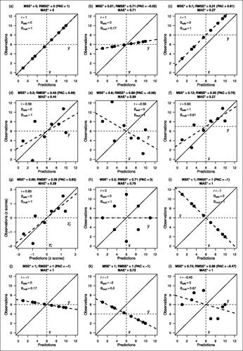
Secondly (Section 4.2), we discuss and visualize the effect of certain characteristics of the data on our new coefficients, and then proceed the other way around and examine what some specific values of the coefficients might tell us about the relationship between predictions and observations. Altogether twelve fictitious data sets are displayed in scatter plot format in Figure 3, and additionally in a time series format in Figure C.1 in the Supplement. In this context, we use the special case of standard scores (z-scores) to visualize the criticism of rescaling the data before calculating an error coefficient in order to eliminate scaling or bias (classified and discussed as type B in Section 2 and Table 3).

Fig. 3 Twelve fictitious sets of n = 8 predicted and observed data illustrate how characteristics of the data (shown inside the boxes) are related to the values of the new coefficients (in the titles). In each panel, the continuous diagonal line is the perfect prediction y = x. The dashed line is the regression line of y on x, drawn to illustrate the difference between high correlation and good prediction. See also Supplementary Table C.1 for details of the data sets and Supplementary Figure C.1 for corresponding “time series formats.”

Thirdly (Section 4.3), we examine the behavior of $\text{MSE*}$ and $\text{MAE*}$ under different types of linear scaling. In this context, we discuss problems of using z-scores and other bias corrections a posteriori. Linear transformations may also be useful for various future applications and research, such as comparing models with different scales, discussing relationships with other normalized coefficients from the literature (Table 3), or for investigating stochastic distributions and estimation problems.

Moreover, in Supplementary Section D we relate our newly normalized coefficient $\text{MSE*}$ to the Taylor diagram (Taylor 2001) which is well-known for visualizing prediction accuracy. The relationship is quite illustrative.

4.1 The normalized coefficients $\text{MSE*}$ and $\text{RMSE*}$ as a function of correlation and biases

To plot the accuracy coefficients as functions of correlation, additive and multiplicative biases, we use eq. (12)(12) $$\text{MSE*}=1-2 \frac{{\mathrm{B}}_{\text{mult}} (1+r)}{{(\frac{{\mathrm{B}}_{\text{add}}}{S_x})}^2+{(1+{\mathrm{B}}_{\text{mult}})}^2}.$$(12) . Figure 2 illustrates the interplay of correlation and biases in their impact on the normalized coefficients $\text{MSE*}$ and $\text{RMSE*}$: In the leftmost column of panels, the coefficients are plotted as functions of correlation and multiplicative bias in the absence of additive bias, in the second column from the left the same but with an additive bias of 1. In the second column from the right, the coefficients are plotted as functions of correlation and additive bias in the absence of multiplicative bias, and in the rightmost column the same but with a multiplicative bias of 2. Apart from the fact that all effects are more pronounced for $\text{RMSE*}$ (bottom row) than for $\text{MSE*}$ (top row) due to the square root, the following pattern is evident in all eight panels: the higher the positive correlation between predictions and observations (r close to 1, see the bottom graphs in all panels), the stronger the effect of biases on the accuracy coefficients. On the other hand, when the correlation is close to 0 or negative (see the upper graphs in all panels), the presence of biases makes almost no difference, i.e. the coefficients are quite high and indicate low prediction accuracy.

Conversely, the lower the biases (see the points near the vertical line in the leftmost column of panels and in the second column from the right), the more the correlation affects the coefficients of prediction accuracy. With increasing biases (see the outer points in the second column from the left and in the rightmost panels), the effect of the correlation decreases.

4.2 Distribution characteristics and coefficient values

How do specific characteristics of the predicted and observed data impact the coefficients $\text{MSE*},\text{RMSE*}$, and $\text{MAE*}$, and how are predicted and observed data related when these new coefficients adopt their minimum, maximum, or halfway between minimum and maximum values? The graphs in Figure 3 illustrate this with some joint distributions of n = 8 predictions and observations. The corresponding prediction accuracy coefficient $\text{PAC}$, a linear transformation of $\text{MSE*}$ which has the same range as the correlation coefficient r, is also given in each panel as it may be more familiar to interpret (see eq. (15)(15) $$\text{PAC}:=1-2·\text{MSE*}.$$(15) ). Possible corresponding time series for each distribution are displayed in Supplementary Figure C.1.

Table C.1 in Supplementary Section C gives the values of the non-normalized coefficients $\text{MSE},\text{RMSE},\text{MAE}$ of the twelve depicted distributions together with their maximum values ${\text{MSE}}_{\mathrm{\text{max}}},{\text{RMSE}}_{\mathrm{\text{max}}}$ and ${\text{MAE}}_{\mathrm{\text{max}}}$ that are possible when considering the given sets of predictions and observations separately, which have been derived in eqs. (7)(7) $$\begin{array}{c}{\text{MSE}}_{\mathrm{\text{max}}}={(\overline{y}-\overline{x})}^2+S_x^2+S_y^2+2 S_x S_y\\ ={(\overline{y}-\overline{x})}^2+{(S_x+S_y)}^2.\end{array}$$(7) and (17)(17) $${\text{MAE}}_{\mathrm{\text{max}}}=|\overline{y}-\overline{x}|+\text{MAD}(x)+\text{MAD}(y),$$(17) and are used for normalization. Table C.1 can be used to illustrate the effects of our new normalization in general: For example, when comparing panels (b) and (d), the $\text{MSE}$ is lower in (b) ($\text{MSE}=6.6$) than in (d) ($\text{MSE}=7.7$), indicating a smaller prediction error, and the $\text{MAE}=2.3$ is equal in (b) and (d). However, as the maximum possible values are much smaller in (b)(${\text{MSE}}_{\mathrm{\text{max}}}=12.9$) than in (d) (${\text{MSE}}_{\mathrm{\text{max}}}=38$, due to larger variance of the observed data), the seemingly better or equal prediction accuracy in (b) vanishes and turns into the contrary when using the new normalized coefficients (e.g., $\text{MSE*}=0.51$ in (b) and 0.20 in (d)), which is apparently more valid when looking at the two time series in Figure C.1. Similar patterns can be found in other panels, for example when comparing (j) to (h).

The panels (a)–(g) of Figure 3 illustrate in particular how specific characteristics of the predicted and observed data impact the new coefficients: The perfect prediction in panel (a) (all observations meet their predictions, so that all new accuracy coefficients denoting error are 0 and $\text{PAC}=1$) is degraded by multiplicative bias in panel (b), additive bias in panel (c), reduced linear correlation in panel (d) and negative correlation in panel (e). Analytically, these three impacts can best be understood with the help of Figure 2 in Section 4.1, which rely on eq. (12)(12) $$\text{MSE*}=1-2 \frac{{\mathrm{B}}_{\text{mult}} (1+r)}{{(\frac{{\mathrm{B}}_{\text{add}}}{S_x})}^2+{(1+{\mathrm{B}}_{\text{mult}})}^2}.$$(12) and plot $\text{MSE*}$ and $\text{RMSE*}$ as functions of biases and correlation. Comparing (b) to (c) shows that the multiplicative bias in (b) affects $\text{MAE*}$ and $\text{RMSE*}$ equally whereas the additive bias in (c) does not. Moreover, the data in (b) illustrate the problem of r as an accuracy coefficient since despite perfect positive correlation, the numerical correspondence of predictions and observations is obviously poor. The large coefficient values $\text{MSE*},\text{RMSE*},\text{MAE*}$ and $\text{PAC}$ close to zero reflect this. Panel (e) shows that a negative correlation of even moderate magnitude leads to coefficients close to their maximum bad values even in the absence of additive or multiplicative bias. This has been formally analyzed in Section 4.1.

Figure 3 panel (f) displays an example without any particularities, rendering it practically the most relevant one. Here, one can see that the farthest outlier from perfect prediction, which occurs at x = 3.5, affects the $\text{RMSE*}$ more than the $\text{MAE*}$.

The impact of z-scaling on the accuracy coefficients is illustrated in panel (g). By z-scaling, the data of a sample are rescaled so that each value denotes its deviation from the sample mean in units of the sample standard deviation (see Supplementary Section A). The resulting standard or z-scores simplify many statistical calculations. Concerning predictions and observations, standardizing both series eliminate all biases and thereby apparently the disadvantage of using r as a measure of prediction accuracy. In panel (g) of Figure 3, the data from panel (f) were z scaled. As a result, the correlation r = 0.83 is unaffected, and the additive and multiplicative biases are removed. In consequence, the coefficients $\text{MSE*},\text{RMSE*}$, and $\text{MAE*}$ are smaller in (g) than in (f) (and $\text{PAC}$ larger), thereby implying a better correspondence of predictions and observations than is actually there. This problem has been mentioned as “artificial skill” in the discussion of bias correction techniques of type (b) in Section 2. (Problems of applying z-scaling and other bias elimination a posteriori in comparative forecast verification and modeling are treated more in-depth in Section 4.3 (iii).)

The panels (a), (h), (i), (j), (k), and (l) of Figure 3, on the other hand, illustrate how predicted and observed data may be related when the new coefficients adopt their minimum, maximum, or halfway between minimum and maximum values. Let us therefore start again with panel (a), where the minimum value 0 of each normalized accuracy coefficient indicates perfect prediction. Figure 3 panels (i-k): The maximum value 1 in the normalized error coefficients indicates the “worst prediction possible.” But what exactly does this mean when using the different coefficients? For the normalizations based on the $\text{MSE}$, it has already been shown in eq. (6)(6) $$\begin{array}{c}\text{MSE}=\overline{d^2}=\overline{d}{ }^2+S_d^2\\ ={(\overline{y}-\overline{x})}^2+S_{y-x}^2\\ ={(\overline{y}-\overline{x})}^2+S_x^2+S_y^2-2 S_x S_y r.\end{array}$$(6) that $\text{MSE*}=\text{RMSE*}=1$ is equivalent to r =–1. Three data examples are shown in the panels (i) (no bias), (j) (multiplicative bias with overdispersed predictions), and (k) (additive bias with overall too large predictions). For $\text{MAE*}=1$, i.e. for $\text{MAE}$ to attain its maximum, it can be seen from eq. (17)(17) $${\text{MAE}}_{\mathrm{\text{max}}}=|\overline{y}-\overline{x}|+\text{MAD}(x)+\text{MAD}(y),$$(17) that two conditions must be met: $$\begin{array}{c}\text{MAE*}=1\iff \text{ MAE}={\text{MAE}}_{\mathrm{\text{max}}}\\ \iff (i)(y_i-\overline{y})(x_i-\overline{x})\le 0\text{ for every i},\text{and}\\ (\mathit{\text{ii}})\overline{y}-\overline{x}=0,\mathrm{i}.\mathrm{e}.{\mathrm{B}}_{\text{add}}\text{=0}.\end{array}$$

The mean absolute error thus attains its maximum if and only if for every data point, the predicted and the observed values lie on opposite sides of their respective mean (non-positive cross product), and there is no additive bias. These conditions are met in panels (i), (j), (l). For comparing $\text{MSE*}$ and $\text{MAE*}$ with regard to their maximum, compare particularly the data set in panel (k), where $\text{MSE*}$ is worst but not $\text{MAE*}$ because of the additive bias, with that in panel (l), where $\text{MAE*}$ is worst but not $\text{MSE*}$ because of each cross product being negative but $r\ne -1$.

Figure 3 panel (h) illustrates one specific example of the “halfway” value $\text{MSE*}=0.5$. It is met if predictions and observations are uncorrelated and the prediction is unbiased (see eq. (12)(12) $$\text{MSE*}=1-2 \frac{{\mathrm{B}}_{\text{mult}} (1+r)}{{(\frac{{\mathrm{B}}_{\text{add}}}{S_x})}^2+{(1+{\mathrm{B}}_{\text{mult}})}^2}.$$(12) ). However, it is easily seen from eq. (12)(12) $$\text{MSE*}=1-2 \frac{{\mathrm{B}}_{\text{mult}} (1+r)}{{(\frac{{\mathrm{B}}_{\text{add}}}{S_x})}^2+{(1+{\mathrm{B}}_{\text{mult}})}^2}.$$(12) that these conditions are sufficient but not necessary, which some other graphs in Figure 3 may roughly illustrate.

4.3 Behavior of MSE* with linear scaling; bias correction a posteriori

Under this heading, we can distinguish different cases with different applications, including the use of z-scores or other bias correction a posteriori. We start with the most general case so that the others are obtained as special cases. $\text{MAE*}$ is only included in the ordinary linear scaling case (ii) because of the less nice mathematical properties of the absolute value function already mentioned above.

1. General linear scaling: Let us linearly rescale the predicted and the observed values with coefficients that are not necessarily identical, i.e.

   ${\tilde{x}}_i=s+t x_i\text{and}{\tilde{y}}_i=u+v y_i.$ (19)

   for some real numbers $s,t,u,v$ with $t,v\ne 0$. Let further $\widetilde{\text{MSE*}}$ denote the normalized $\text{MSE*}$ for the rescaled variables. With the familiar linear scaling rules for mean, standard deviation, and covariance (eqs. (A.1), (A.3), (A.8) in the Glossary in the Supplement), we use the expression in eq. (9)(9) $$\text{MSE*}=1-2 \frac{S_x S_y+S_{\mathit{\text{xy}}}}{(\overline{y}-\overline{x}){ }^2+{(S_x+S_y)}^2}.$$(9) to arrive at

   $\widetilde{\text{MSE*}}=1-2 \frac{\left|t\right|\left|v\right|S_x S_y+\mathit{\text{tv}} S_{\mathit{\text{xy}}}}{{(u+v\overline{y}-s-t\overline{x})}^2+{(|t|S_x+|v|S_y)}^2}.$ (20)

2. Ordinary linear scaling: Since x and y denote the same physical quantity, predicted and observed, in most cases they are being rescaled with identical linear coefficients. This applies when we want to transform our variable for comparing prediction accuracy across studies using different scales, e.g. degrees Fahrenheit and degrees Celsius. With s = u and t = v in eq. (19), eq. (20) reduces to

   $\begin{array}{c}\widetilde{\text{MSE*}}=1-2 \frac{\left|v\right|\left|v\right|S_x S_y+\mathit{\text{vv}} S_{\mathit{\text{xy}}}}{{(u+v\overline{y}-u-v\overline{x})}^2+{(|v|S_x+|v|S_y)}^2}\\ =1-2 \frac{S_x S_y+S_{\mathit{\text{xy}}}}{\overline{d}{ }^2+{(S_x+S_y)}^2}\\ =\text{MSE*}.\end{array}$ (21)

   $\text{MSE*}$ and $\text{RMSE*}$ are therefore invariant against ordinary linear scaling. The same holds for $\text{MAE*}$, which can be shown by analogy. (Note that the invariance of $\text{MSE*}$ against ordinary linear scaling could likewise be obtained by applying the definition (eq. (8)(8) $$\begin{array}{c}\text{MSE*}:=\frac{\text{MSE}}{{\text{MSE}}_{\mathrm{\text{max}}}}\\ =\frac{\frac{1}{n}\sum _{i=1}^n{(y_i-x_i)}^2}{{(\overline{y}-\overline{x})}^2+{(S_x+S_y)}^2}\\ =\frac{\overline{d^2}}{\overline{d}{ }^2+{(S_x+S_y)}^2}.\end{array}$$(8) ) to the linearly transformed variables.)

3. Unbiased prediction; z-scores and other bias correction a posteriori: If the prediction is additively and multiplicatively unbiased, i.e. predicted and observed values have identical means and variances, then $\text{MSE*}$ is a simple linear transformation of the correlation r, and the two coefficients can be used interchangeably to assess the prediction accuracy (see eq. (13)(13) $$\text{MSE*}=\frac{1-r}{2}.$$(13) , repeated here for clarity):

   $\text{MSE*}=0.5 (1-r),\text{RMSE*}=\sqrt{0.5 (1-r)}\text{and PAC}=r.$ (22)

A special linear transformation for equalizing means and variances and thereby eliminating biases is the use of z-scores, which are computed separately for predictions and observations. A z-score of a data point in an empirical data set denotes its difference from the arithmetic mean in units of the standard deviation of the data set, which implies a mean of zero and a variance and standard deviation of one (see the definition in Supplementary Subsection A.5 and eqs. (A.12), (A.13) therein). With zero means and unit variances in predictions and observations, the prediction is by definition unbiased and the $\text{MSE*}$ of the z-scores is a linear function of their correlation $r_{z_x{z}_y}$. This correlation $r_{z_x{z}_y}$ is also the slope of the regression line when performing the linear regression of observed on predicted z-scores or vice versa, and equal to the correlation r_xy of original predictions and observations (see eqs. (A.14), (A.15) in the Supplement; the reader might use Figure 1 and Figure 3 panel (g) for visualisation). However, despite all statistical simplicity, we would like to emphasize that in the prototypical situation in which one would want to use normalized accuracy coefficients, namely for assessing prediction accuracy, the result in eq. (13)(13) $$\text{MSE*}=\frac{1-r}{2}.$$(13) shows that any such de-biasing, including z-scaling, yields an artificial accuracy (“spurious skill”). In other words, eliminating all biases precludes diagnosing them. Since predictions and observations are transformed separately, the $\text{MSE*}$ (and also the $\text{RMSE*}$ and $\text{MAE*}$) are usually smaller, thus apparently better, with z-scores than with the original data (see eq. (20), Figure 3 panels (g) vs. (f), and the corresponding Table C.1 in the Supplement).

A more general bias correction a posteriori, i.e. after predictions and observations have been obtained, is given by eq. (23)(23) $${\tilde{x}}_i=\frac{S_y}{S_x} x_i+(\overline{y}-\frac{S_y}{S_x} \overline{x}),$$(23) below: The predictions are rescaled using means and standard deviations so that multiplicative and additive biases are removed: (23) $${\tilde{x}}_i=\frac{S_y}{S_x} x_i+(\overline{y}-\frac{S_y}{S_x} \overline{x}),$$(23) implying $S_{\tilde{x}}^2=S_y^2$ and $\overline{\tilde{x}}=\overline{y}$ because of the familiar linear scaling rules for means and variances (eqs. A.1(10) $${\mathrm{B}}_{\text{add}}=\overline{d}=\overline{y}-\overline{x}.$$(10) and A.2 in the Supplemental Material). Obviously, this rescaling produces similar artificially low coefficients $\text{MSE*},\text{RMSE*}$, and $\text{MAE*}$ as the z-scaling. We have written this paragraph mainly in order to discourage such attempts. (That even more sophisticated a posteriori bias-correction techniques such as cross-correlation almost inevitably lead to artificial measures of accuracy, has been extensively discussed in the literature (e.g. Dequé 2012; Maraun and Widmann 2018) and has been mentioned above in Section 2).

5 Application: case study

As mentioned in the introduction (Table 2), the new normalized coefficients of prediction accuracy are particularly beneficial for comparative forecast verification and modeling if two conditions are met: First, the data consists of data sets with different scales (otherwise, the unit-dependent coefficients $\text{MSE},\text{ RMSE}$ or $\text{MAE}$ were applicable and comparable between data sets without problems). Second, the predictions are not obtained from the observations by a linear least-squares model fit (otherwise, r and R² could be used because additive and multiplicative biases were excluded). With a data example from atmospheric sciences we demonstrate the advantages of our new normalized coefficients $\text{RMSE*}$ and $\text{PAC}$ over the classic $\text{RMSE}$ and r in such conditions.

5.1 Data

We employed singular spectrum analysis (SSA, Golyandina et al. 2001, 2018) in an attempt to forecast monthly rainfall in African countries based on past rainfall. Although the attempt itself failed in most parts, the results are well suited to compare the performance of $\text{RMSE*}$ and $\text{PAC}$ with that of $\text{RMSE}$ and r in forecast verification because almost the entire range of coefficient values occurred. Here we present forecasts of monthly rainfall in Ethiopia for the years 1978–1985, based on SSA rainfall reconstructions for the years 1920–1977.

Both of the above conditions were met: First, the data consist of twelve monthly rainfall subsets scaled differently (see six example months in Figure 4). Second, the forecasts were produced by SSA and not by linear least squares modeling of the observations, so additive and multiplicative prediction biases may well occur.

Fig. 4 Monthly rainfall series from Ethiopia in the years 1920–1985 for six selected months of the year with different levels of rainfall (January, February, March, May, October, December). SSA decomposition and reconstruction was applied to the data to the left of the vertical line (58 years, 1920–1977). SSA forecast was applied to the data to the right of the vertical line (eight years, 1978–1985). The black dots indicate the observed monthly rainfall (CRU 2022), the white dots the reconstructed (left) and the forecast (right) monthly rainfall.

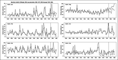
The rainfall data were taken from the Climatic Research Unit of the University of East Anglia (2022), using Harris et al. (2020). All calculations and plots were conducted with R (R Core Team 2022).

5.2 Method

The basic aim of SSA is to decompose a time series into a sum of meaningful components plus noise without making assumptions about a parametric form of these components (Golyandina et al. 2001). From this composition, on the one hand the hypothetical time series without noise can be reconstructed, and on the other hand it can be extrapolated into the future to provide a forecast. In basic SSA, two parameters determine the result, i.e. which variation of the data is considered meaningful and which is considered noise: L, the so-called window length, and d, the number of eigenvectors considered (number of additive components). Since a numerical determination of L and d, i.e. a classical model fit, is not possible (in the extreme case the noise can always be set to zero), pragmatic criteria have been established: For the window length L, (Golyandina et al. 2018, ch. 2.1.3.2, 2.1.5.1) recommend to choose about half the length of the time series. For d, there is a tradeoff between a good reconstruction (the larger d the better) and its meaningfulness and predictive power if there is regularity in the data (too large a d-value is counterproductive).

Of the two applications of our new coefficients, comparative forecast verification and modeling, only the first is shown in this case study. As required for SSA forecast verification, the data sample was split into two time periods: The years 1920-1977 were used to run the SSA on the twelve monthly rainfall series with the parameters L and d set equally for all months, namely L = 29, half the length of the time series as recommended, and d = 7. With the obtained decomposition of the time series, we forecast (or better, hindcast) the monthly rainfall for the years 1978–1985. For this forecast period, we assessed the agreement between the forecasts and the observations on the one hand with the classic coefficients of forecast accuracy $\text{RMSE}$ and r, and on the other hand with our new normalized coefficients $\text{RMSE*}$ and the $\text{PAC}$ (as mentioned, the latter ranges from–1 to 1, which allows a more familiar interpretation analogous to r). In order to assess the adequacy of each coefficient for comparative forecast verification, we adopted a rather intuitive approach, well aware that it entails the risk of circular reasoning (the reader is invited to judge this by scrutinizing the results presented below): For every pair of predicted versus observed data, we separately determined the additive bias ${\mathrm{B}}_{\text{add}}$, the multiplicative bias ${\mathrm{B}}_{\text{mult}}$, and the “progression similarity” r, which we regarded to be the relevant components of agreement (see Section 4.1), and then discussed how these components were reflected in the coefficient values obtained for each of the 12 monthly rainfall series. We also calculated some coefficients proposed in the literature for normalization and de-biasing (see Table 3), namely the normalized mean square errors NMSE (Pokhrel and Gupta 2010) and the NMSE’ (Gupta and Kling 2011), the mean squared error skill score MSESS (Dequé 2012) using the 1920–1949 average as reference, and the mean absolute percentage error MAPE (Armstrong and Collopy 1992), and examined whether the issues of criticism reviewed in Section 2 were visible in the rainfall data.

5.3 Results and discussion

Figure 4 shows the monthly rainfall series in Ethiopia and the SSA results for the two periods, the years 1920-1977 (SSA reconstruction) and the years 1978–1985 (SSA forecast) in six selected months of the year. The ordinates show that the series are scaled differently: rainfall in December, January and February is much lower than in May and October. The six months have been selected for illustration because here, the forecasts exhibit the most interesting characteristics where our new normalized coefficients show their superiority, and/or where the problems of some of the normalizations from the literature become visible. This is further detailed in Table 4, which covers all months of the year, and in Figure 5, which is related to the theoretical discussion in Section 4.2 and corresponds in format to Figure 3.

Fig. 5 Joint distributions of predicted (SSA forecast, better: hindcast) and observed monthly rainfall in Ethiopia in the years 1978–1985, together with components of prediction accuracy (inside the graph areas) and coefficient values (in the titles). The forecasts were obtained from SSA with L = 29 and d = 7 in the years 1920–1977. The observations were from Climatic Research Unit of the University of East Anglia (2022).

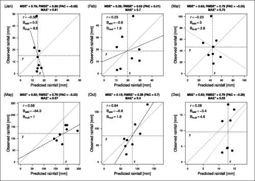
Table 4 Comparative verification of the SSA forecast of monthly Ethiopian rain in the years 1978–1985.

Month	${\mathrm{B}}_{\text{add}}$	${\mathrm{B}}_{\text{mult}}$	r	$\text{RMSE}$	RMSE*	PAC	$\text{MAE}$	MAE*	NMSE	NMSE’	MSESS	MAPE
Jan	0.5	8.63	−0.38	14.9	0.89	-0.58	11.5	0.91	1.10	9.51	0.03	178.5
Feb	−0.8	1.87	0.23	14.3	0.63	0.21	13.3	0.70	1.05	1.95	−0.04	120.3
Mar	3.0	2.80	−0.23	27.4	0.79	-0.25	20.7	0.75	1.31	3.66	−0.30	53.0
Apr	−19.2	1.72	0.24	35.9	0.68	0.08	25.4	0.43	1.48	2.55	−0.48	44.3
May	−64.3	0.97	0.58	69.5	0.78	-0.23	64.3	0.57	6.01	5.83	−4.85	59.3
Jun	−12.1	1.50	0.40	18.6	0.65	0.16	16.7	0.53	1.59	2.39	0.15	28.1
Jul	−16.5	1.80	−0.28	25.7	0.85	-0.43	22.9	0.64	2.76	4.95	−0.72	22.1
Aug	−30.3	1.19	−0.11	45.1	0.80	-0.28	31.1	0.46	3.44	4.08	−1.10	33.4
Sep	−8.4	1.53	0.24	15.0	0.67	0.09	10.9	0.42	1.63	2.48	0.28	12.7
Oct	−6.8	1.86	0.84	27.5	0.39	0.70	23.8	0.40	0.40	0.75	0.61	47.5
Nov	−24.7	0.78	0.75	29.4	0.57	0.36	27.1	0.49	2.41	1.88	−1.24	111.7
Dec	−3.4	4.62	0.28	6.6	0.79	-0.26	5.6	0.55	1.24	5.75	−0.22	124.7

Columns 2–4 show components of agreement between predicted and observed data. Columns 4–5 contain the values of two classic coefficients of prediction accuracy (r and $\text{RMSE}$). Columns 6–7, bold face, show the values of two of our new normalized coefficients of prediction accuracy; note that $\text{RMSE*}$ is an error score, i.e. 0 is best and 1 is worst, while $\text{PAC}$ is an accuracy score bound between–1 = worst and 1 = best. Columns 8–9 compare the classic $\text{MAE}$ with its new normalised form $\text{MAE*}$. Finally, columns 10–13 show the values of some “normalizations” from the literature: NMSE and NMSE’ are error scores without upper bounds, MSESS is a skill score indicating the proportional improvement over a forecast using the 1920–1949 average, and MAPE is a percentage error score without upper bound.

We restrict this discussion to the six monthly series depicted in Figures 4 and 5, as these are sufficient to show the advantages of the new normalized error coefficient $\text{RMSE*}$ and accuracy coefficient $\text{PAC}$. After discussing these months individually, we examine where the advantages and disadvantages of the normalizations from the literature show up in the data.

The forecast of January rainfall (first panels in Figures 4 and 5) failed most prominently. This shows in a multiplicative bias of more than 8 (the observed rain varied eight times more than the predicted, largely due to an outlier in the observations), and a negative correlation between predictions and observations. Accordingly, the $\text{RMSE*}$ and the $\text{MAE*}$ are close to their maximum, and the $\text{PAC}=-0.58$. The $\text{PAC}$ is more negative than $r=-0.38$ and reflects thereby not only the reverse course of predictions and observations, as r does, but additionally the adverse multiplicative bias.

In February, the predictions are almost unbiased and thereby not as bad as in January, but nevertheless they are of limited use because their course does not resemble that of the observations (r = 0.23). Whereas the classic $\text{RMSE}$ does not indicate this superiority over January (both $\text{RMSE}\approx 14$), $\text{RMSE*}$ does, and even more so $\text{PAC}$, which is strongly negative in January and slightly positive in February.

March is the only month where the predictions underestimate the observations, i.e. the additive bias $\overline{y}-\overline{x}$ is slightly positive. Moreover, the predictions are poor as they are underdispersed (B_mult > 2) and the course runs contrary to that of the observations (r < 0). This is reflected in a very high $\text{RMSE*}$ and $\text{MAE*}$, and a negative $\text{PAC}$, although even the classic coefficients were able to detect the failure. We have included this month because it is interesting in the discussion of the normalizations from the literature below.

For May, the predicted and the observed rainfall series run similarly in the forecast period, almost parallel, but with a very large negative additive bias (on average, about 64 mm less rainfall was observed than predicted). The quite high value of r = 0.58, however, does not reflect this practically useless prediction. In contrast, $\text{RMSE*}=0.78$ and $\text{PAC}=-0.23$ reveal that the forecast had failed, and (to a slightly lesser degree) also $\text{MAE*}=0.57$.

October rainfall was predicted well by the SSA. This can be seen from the progression similarity of the time courses in the forecast period in Figure 4, even covering outliers, and in the quite small additive and multiplicative biases (Table 4). Accordingly, the high correlation r = 0.84 is almost preserved in the coefficient values $\text{RMSE*}=0.39,\text{MAE*}=0.40$ (small values are “good”) and $\text{PAC}=0.70$. October is the only month in which the SSA forecast succeeded. The classic $\text{RMSE}=27.5$ and $\text{MAE}=23.8$ were almost the same as for March ($\text{RMSE}=27.4,\text{ MAE}=20.7$) and could thus not indicate this success, whereas in the absence of biases, the classic r could.

December is interesting because the overall rainfall level is very low, on average less than 10 mm (Figure 4). The absolute values of $\text{RMSE}$ and $\text{MAE}$ thus look good (last line of Table 4). However, the standard deviation of the observations is more than four times as large as that of the predictions (high multiplicative bias), and together with a negligible correlation, the prediction is in fact useless (compare predicted and observed rainfall in the forecast period in the last panels of Figures 4 and 5). And whereas r is positive albeit small, the complete failure of the forecast becomes evident only from the high $\text{RMSE*}$ (close to maximum), to a slightly lesser degree the high $\text{MAE*}$, and the negative $\text{PAC}$ values.

In the last four columns of Table 4, we evaluated four coefficients proposed in the literature to eliminate scaling and/or bias. Referring to our categorization in Section 2, two are in category A.1, i.e. use measures from the sample data to normalize the original error coefficient: The normalized mean square errors NMSE (Pokhrel and Gupta 2010) normalizes the $\text{MSE}$ at the variance of the observations, and the NMSE’ (Gupta and Kling 2011) normalizes it at the product of standard deviations of the predictions and observations. Both are able to diagnose the success of the October forecast, as their values here are by far the lowest here (0.40 and 0.75). However, the blatant failure of the January forecast is not detected by the NMSE, which gives the third best value of all months here. Obviously, this is due to the outlier and the correspondingly large variance of the observations, by which the $\text{MSE}$ is divided and an artificially small value of the NMSE is produced. This illustrates well the criticism made by Ehret and Zehe (2011). The NMSE’ does not suffer from this disadvantage, as its January value is the worst of all the months. In fact, the ranking of its values almost perfectly matches that of $\text{RMSE*}$ and (inversely) the $\text{PAC}$. The only drawback is that there is no upper limit, which leads to a distortion of the values, as reflected in the disproportionately high January value of 9.51.

With the MSESS (Dequé 2012), we also evaluated one coefficient from category A.2, which are skill scores that use measures from past data to normalize the original error coefficient. The MSESS is bounded between 0 and 1, and gives the proportional improvement of the current prediction over a constant prediction made by the average of the reference period. If the current data have generally changed relative to the reference, as in climate change, a “spurious,” i.e. apparent, skill is produced (Fricker et al. 2013). Since in our rainfall data, almost no climatic change is visible, we used the earliest years in the sample 1920–1949 as reference period and could show at least a small spurious skill in the September data (see Table 4): The apparent improvement by 28% might be due to an average reduction in rainfall (96 mm for 1978–1985, compared to 109 mm for 1920–1949) rather than a success of the forecasting model. The MSESS also appeared to be problematic in that it was unable to detect the blatant failure of the January forecast (MSESS = 0.03), instead stating that the November (MSESS =–1.24) and March (MSESS =–0.30) forecasts were much worse, which is not reflected in the data.

Finally, we evaluated one of the coefficients from category B.1 (where each pair of data is individually normalized before the coefficient is calculated), namely the mean absolute percentage error MAPE (Armstrong and Collopy 1992). Since the prediction error at each point is divided by the observed value (see Table 3), overestimates (negative additive bias) are penalized more than underestimates (positive additive bias). In our data, this is evident when comparing March and December: While our new coefficients $\text{RMSE*}=0.79/0.79$ and $\text{PAC}=-0.25/-0.26$ are both (almost) equal here, indicating equally bad forecasts in March and December, according to MAPE the unsuccessful March forecast (MAPE = 53) is almost as good as the really successful October forecast (MAPE = 47.5), while the December forecast (MAPE = 124.7) is more than twice as bad. This does not agree with the picture in Figure 5. Moreover, the best forecast according to MAPE is the September forecast (MAPE = 12.7), which is not at all supported by the data in Table 4.

To sum up, we have illustrated with six examples of comparative forecast verification that our new normalized coefficients $\text{RMSE*},\text{MSE*}$, and $\text{PAC}$ reflected all points of prediction accuracy (biases and course), which neither the $\text{RMSE}$ (and its monotonically related concepts) nor the correlation r were able to do. Other normalizations proposed in the literature have advantages in some areas, but in our examples of comparative forecast verification the drawbacks already mentioned in the literature have become apparent.

6 Conclusions and discussion

This paper deals with the evaluation of forecasts or predictions of univariate numerical data consisting of subsets with different scales. In this situation, the classical unit-dependent error coefficients $\text{MSE},\text{ RMSE},$ or $\text{MAE}$ are not applicable.

We have developed new normalizations of these classical coefficients: The normalized mean squared error $\text{MSE*}$, its root $\text{RMSE*}$, and the normalized mean absolute error $\text{MAE*}$. They range between 0 (indicating perfect prediction) and 1 (indicating the maximum $\text{MSE},\text{ RMSE}$ or $\text{MAE}$ value that is possible when the two series of data at hand, predicted and observed, are considered separately, regardless of their pairing). The idea is the same as in calculating the correlation r as a normalized covariance. We also suggest an alternative form of the $\text{MSE*}$, the prediction accuracy coefficient $\text{PAC}$, which ranges between–1 and 1. It may become popular because its interpretation is familiar to that of the correlation coefficient r, and even equals r if the data are standard scores (z-scaled).

In a variety of disciplines, the problems of forecast verification or modeling using differently scaled data are well known. In response to these problems, the various disciplines have developed a variety of normalizations and other modifications of the classic coefficients of prediction accuracy $\text{MSE},\text{ RMSE},\text{ MAE}$, and r. However, almost all of these modifications either treat the two sets of data, predicted and observed, asymmetrically, or rely on past data, both of which may introduce new bias and artificial skill. Our $\text{MSE*},\text{RMSE*},\text{MAE*}$, and $\text{PAC}$ avoid these two clusters of problems in comparative forecast verification and modeling. In the present paper, we have examined some properties of the new coefficients algebraically and empirically, the latter using small artificial datasets and a case study. In particular, we have shown that our new coefficients account well for three conditions in the data that are necessary for good agreement between predicted and observed data: The absence of an additive bias, the absence of a multiplicative bias, and a similar trajectory of ups and downs over time or space.

There are two very different research scenarios for which we particularly recommend our new coefficients: The first is what we call “comparative forecast verification.” This involves forecasting future data for subsets with different scales and evaluating the forecast with later observations. Here we propose our new coefficients without any restrictions. The second is what we call “comparative modeling.” Here the predictions do not concern the future, but represent a model fit to observations consisting of subsets with different scales. The coefficients are used to assess the agreement between predictions and observations in the process of model fitting, i.e. choosing model parameters so that the coefficients indicate an optimal fit. In this scenario, our new normalized coefficients are only necessary if the predictions are made other than by linear least-squares modeling of the observations, because for linear least-squares models one can use the well-known R² or r to optimize the fit.

In brief, the typical application for our new coefficients is a case where two conditions meet: The data consists of subsets with different scales, and the predictions are not made by a linear least-squares model fit of the observations (which is trivially the case in comparative forecast verification). Such a typical application case was chosen in Section 5 to demonstrate the advantages of our new coefficients on a data example from atmospheric science.

Further work is needed to establish the coefficients in practice in the various disciplines. First, their properties and behavior under different conditions should be studied in more detail, for example with simulated data. Second, their relationship to existing ideas of normalization or modification of the coefficients $\text{MSE},\text{ RMSE},\text{ MAE}$ and r needs to be investigated both mathematically and empirically. In the present paper, we have only given a rough overview of the literature on such approaches, and have not gone into depth. Third, the stochastic properties of our new coefficients need to be studied, with or without assumptions about the distribution of the random variable from which we assume our finite data sample was drawn. Bootstrapping might be a good place to start with the latter.

Acknowledgments

The authors would like to thank Dieter Heyer, Svetlana Wähnert, and Eike Richter for their valuable feedback on previous versions of this paper. They are especially grateful to Richard Gross for his meticulous proofreading, which improved the English language and eliminated ambiguities.

Disclosure statement

All authors declare that they have no conflicts of interest.

Data availability statement

The data that support the findings of the case study (Section 5) are openly available in figshare at http://doi.org/10.6084/m9.figshare.23284373.

Additional information

Funding

We acknowledge support by the German Research Foundation and the Open Access Publication Fund of TU Berlin.

References

- Abe, CF, Dias, JB, Notton, G, Faggianelli, GA. 2020. Experimental application of methods to compute solar irradiance and cell temperature of photovoltaic modules. Sensors 20(9):2490.
- Afshar K, Bigdeli N. 2011. Data analysis and short term load forecasting in Iran electricity market using singular spectral analysis (SSA). Energy 36(5):2620–2627.
- Armstrong JS, Collopy F. (1992). Error measures for generalizing about forecasting methods: Empirical comparisons. Int J Forecast. 8(1):69–80.
- Audrino F, Sigrist F, Ballinari D. 2020. The impact of sentiment and attention measures on stock market volatility. Int J Forecast. 36(2):334–357.
- Burrows SM, Dasgupta A, Reehl S, Bramer L, Ma P-L, Rasch PJ, Qian Y. 2018. Characterizing the relative importance assigned to physical variables by climate scientists when assessing atmospheric climate model fidelity. Adv Atmos Sci 35(9):1101–1113.
- Campbell JY, Thompson SB. 2008. Predicting excess stock returns out of sample: Can anything beat the historical average? Rev Financ Stud. 21(4):1509–1531.
- Cantelmo G, Kucharski R, Antoniou C. 2020. Low-dimensional model for bike-sharing demand forecasting that explicitly accounts for weather data. Transp Res Record: J Transp Res Board 2674(8):132–144.
- Chen, D, Rojas, M, Samset, BH, Cobb, K, Diongue-Niang, A, Edwards, P, Emori, S, Faria, SH, Hawkins, E, Hope, P, et al. 2021. Framing, context, and methods. In: Masson-Delmotte V, Zhai P, Pirani A, Connors SL, Péan C, Berger S, Caud N, Chen Y, Goldfarb L, Gomis MI, et al. editors. Climate Change 2021: The Physical Science Basis. Contribution of Working Group I to the Sixth Assessment Report of the Intergovernmental Panel on Climate Change. Cambridge (UK); New York (NY): Cambridge University Press. p. 147–286.
- Climatic Research Unit of the University of East Anglia. 2022. High-resolution gridded datasets (and derived products). CRU CY v4.06 Country Averages: PRE; [accessed 2022 Sep 12]. https://crudata.uea.ac.uk/cru/data/hrg/cru_ts_4.06/crucy.2205251923.v4.06/countries/pre/.
- Daetwyler HD, Villanueva B, Woolliams JA. 2008. Accuracy of predicting the genetic risk of disease using a genome-wide approach. PLoS ONE 3(10):e3395.
- Daum SO, Hecht H. 2009. Distance estimation in vista space. Atten Percept Psychophys. 71(5):1127–1137.
- Dequé M. 2012. Deterministic forecasts of continuous variables. In Jolliffe IT, Stephenson DB, editors, Forecast verification. A pracitioner’s guide in atmospheric science. Hoboken (NJ): Wiley. p. 77–94.
- Ehret U, Zehe E. 2011. Series distance–an intuitive metric to quantify hydrograph similarity in terms of occurrence, amplitude and timing of hydrological events. Hydrol Earth Syst Sci. 15(3):877–896.
- Engbert R, Nuthmann A, Richter EM, Kliegl R. 2005. SWIFT: a dynamical model of saccade generation during reading. Psychol Rev. 112(4):777–813.
- Fricker TE, Ferro CAT, Stephenson DB. 2013. Three recommendations for evaluating climate predictions. Meteorol Appl. 20(2):246–255.
- Gneiting T. 2011. Making and evaluating point forecasts. J Amer Stat Assoc. 106(494):746–762.
- Goelzer H, Nowicki S, Edwards T, Beckley M, Abe-Ouchi A, Aschwanden A, Calov R, Gagliardini O, Gillet-Chaulet F, Golledge NR, et al. 2018. Design and results of the ice sheet model initialisation experiments initMIP-Greenland: an ISMIP6 intercomparison. Cryosphere. 12(4):1433–1460.
- Goldberg K, Roeder T, Gupta D, Perkins C. 2001. Eigentaste: A constant time collaborative filtering algorithm. Inf Retr. 4(2):133–151.
- Golyandina N, Korobeynikov A, Zhigljavsky A. 2018. Singular spectrum analysis with R. Berlin: Springer.
- Golyandina N, Nekrutkin V, Zhigljavsky AA. 2001. Analysis of time series structure: SSA and related techniques. Boca Raton, FL: Chapman and Hall/CRC.
- Gupta HV, Kling H. 2011. On typical range, sensitivity, and normalization of mean squared error and Nash-Sutcliffe efficiency type metrics. Water Resour Res. 47(10):W10601.
- Gupta HV, Kling H, Yilmaz KK, Martinez GF. 2009. Decomposition of the mean squared error and NSE performance criteria: Implications for improving hydrological modelling. J Hydrol 377(1–2):80–91.
- Gustafson WI, Yu S. 2012. Generalized approach for using unbiased symmetric metrics with negative values: Normalized mean bias factor and normalized mean absolute error factor. Atmos Sci Lett. 13(4):262–267.
- Hammi O, Miftah A. 2015. Complexity-aware-normalised mean squared error ‘CAN’ metric for dimension estimation of memory polynomial-based power amplifiers behavioural models. IET Commun. 9(18):2227–2233.
- Harris I, Osborn TJ, Jones P, Lister D. 2020. Version 4 of the CRU TS monthly high-resolution gridded multivariate climate dataset. Sci Data 7(1):109.
- Hyndman RJ, Athanasopoulos G. 2021. Forecasting: principles and practice. OTexts, 3rd ed.
- Hyndman RJ, Koehler AB. 2006. Another look at measures of forecast accuracy. Int J Forecast 22(4):679–688.
- Istas J. 2005. Mathematical modeling for the life sciences. Berlin: Springer.
- Jacobs DA, Ferris DP. 2015. Estimation of ground reaction forces and ankle moment with multiple, low-cost sensors. J NeuroEng Rehabil. 12(1):1–12.
- Khain AP, Beheng KD, Heymsfield A, Korolev A, Krichak SO, Levin Z, Pinsky M, Phillips V, Prabhakaran T, Teller A, et al. 2015. Representation of microphysical processes in cloud-resolving models: Spectral (bin) microphysics versus bulk parameterization. Rev Geophys. 53(2):247–322.
- Krause P, Boyle DP, Bäse F. 2005. Comparison of different efficiency criteria for hydrological model assessment. Adv. Geosci. 5:89–97.
- Legates DR, McCabe GJ. 1999. Evaluating the use of “goodness-of-fit” measures in hydrologic and hydroclimatic model validation. Water Resour Res. 35(1):233–241.
- Li J. 2017. Assessing the accuracy of predictive models for numerical data: Not r nor r2, why not? then what? PLoS ONE 12(8):e0183250.
- Magnusson L, Ackerley D, Bouteloup Y, Chen J-H, Doyle J, Earnshaw P, Kwon YC, Köhler M, Lang STK, Lim Y-J, et al. 2022. Skill of medium-range forecast models using the same initial conditions. Bull Amer Meteorol Soc. 103(9):E2050–E2068.
- Makridakis S, Hibon M. 2000. The M3-competition: results, conclusions and implications. Int J Forecast 16(4):451–476.
- Maraun D, Widmann M. 2018. Cross-validation of bias-corrected climate simulations is misleading. Hydrol Earth Syst Sci. 22(9):4867–4873.
- Mauritsen T, Roeckner E. 2020. Tuning the MPI-ESM1.2 global climate model to improve the match with instrumental record warming by lowering its climate sensitivity. J Adv Model Earth Syst. 12(5):e2019MS002037.
- Mauritsen T, Stevens B, Roeckner E, Crueger T, Esch M, Giorgetta M, Haak H, Jungclaus J, Klocke D, Matei D, et al. 2012. Tuning the climate of a global model. J Adv Model Earth Syst. 4(3):M00A01.
- Müller-Plath G, Ott DVM, Pollmann S. 2010. Deficits in subprocesses of visual feature search after frontal, parietal, and temporal brain lesions—a modeling approach. J Cogn Neurosci. 22(7):1399–1424.
- Müller-Plath G, Pollmann S. 2003. Determining subprocesses of visual feature search with reaction time models. Psychol Res. 67(2):80–105.
- Murphy AH. 1988. Skill scores based on the mean square error and their relationships to the correlation coefficient. Monthly Weather Rev. 116(12):2417–2424.
- Nash JE, Sutcliffe JV. 1970. River flow forecasting through conceptual models part I - A discussion of principles. J Hydrol. 10(3):282–290.
- Norman JF, Adkins OC, Pedersen LE. 2016. The visual perception of distance ratios in physical space. Vis Res. 123:1–7.
- Nossent J, Bauwens W. 2012. Application of a normalized Nash-Sutcliffe efficiency to improve the accuracy of the Sobol’ sensitivity analysis of a hydrological model. In: EGU General Assembly Conference Abstracts, EGU General Assembly Conference Abstracts. p. 237.
- Otto SA. 2019. How to normalize the RMSE [blog post]; [accessed 2023 Oct 23]. https://www.marinedatascience.co/blog/2019/01/07/normalizing-the-rmse/.
- Pokhrel P, Gupta HV. 2010. On the use of spatial regularization strategies to improve calibration of distributed watershed models. Water Resour Res. 46(1):W01505.
- Potts JM. 2012. Basic concepts. In: Jolliffe IT, Stephenson DB, editors. Forecast verification. A pracitioner’s guide in atmospheric science. Hoboken, NJ: Wiley, p.11–30.
- Previsic, M, Karthikeyan, A, Lyzenga, D. 2021. In-ocean validation of a deterministic sea wave prediction (DSWP) system leveraging X-band radar to enable optimal control in wave energy conversion systems. Appl Ocean Res. 114:102784.
- R Core Team. 2022. R: a language and environment for statistical computing. Vienna, Austria: R Foundation for Statistical Computing.
- Rahman MH, Salma U, Hossain MM, Khan MTF. 2016. Revenue forecasting using Holt-Winters exponential smoothing. Res Rev J Stat. 5(3):19–25.
- Stephen KD, Kazemi A. 2014. Improved normalization of time-lapse seismic data using normalized root mean square repeatability data to improve automatic production and seismic history matching in the Nelson field. Geophys Prospect. 62(5):1009–1027.
- Taylor KE. 2001. Summarizing multiple aspects of model performance in a single diagram. J Geophys Res Atmos. 106(D7):7183–7192.
- Van Zandt T, Townsend JT. 2012. Mathematical psychology. In: Cooper H, Camic PM, Long DL, Panter AT, Rindskopf D, Sher KJ, editors. APA handbook of research methods in psychology, Vol 2: research designs: quantitative, qualitative, neuropsychological, and biological. American Psychological Association.
- Von Storch H, Zwiers FW. 2002. Statistical analysis in climate research. Cambridge: Cambridge University Press.
- Voudouri A, Avgoustoglou E, Carmona I, Levi Y, Bucchignani E, Kaufmann P, Bettems J-M. 2021. Objective calibration of numerical weather prediction model: application on fine resolution COSMO model over Switzerland. Atmosphere 12(10):1358.
- Waldmann P. 2019. On the use of the Pearson correlation coefficient for model evaluation in genome-wide prediction. Front Genet. 10:899.
- Wilks D. 2019. Statistical methods in the atmospheric sciences, 4th ed. Amsterdam: Elsevier.
- Willmott CJ. 1981. On the validation of models. Phys Geogr. 2(2):184–194.
- Willmott CJ, Ackleson SG, Davis RE, Feddema JJ, Klink KM, Legates DR, O’Donnell J, Rowe CM. 1985. Statistics for the evaluation and comparison of models. J Geophys Res. 90(C5):8995–9005.
- World Meteorological Organization. 2019. Manual on the Global Data-processing and Forecasting System (WMO-No. 485): Annex IV to the WMO Technical Regulations. World Meteorological Organization. updated in 2022.
- World Meteorological Organization. 2023. WMO Lead Centre for Deterministic NWP Verification (LC-DNV). Lead Centre guidelines. Score definitions and requirements; [accessed 2023 Oct 23]. https://confluence.ecmwf.int/display/WLD/Score+definitions+and+requirements.
- Zambresky L. 1989. A verification study of the global WAM model December 1987 - November 1988. Techreport 63, GKSS Forschungszentrum, Federal Republic of Germany.