Design and hydrodynamic analysis of controllable soft-body extension-driven flippers inspired by swimming frog flippers

Abstract

Flippers are key tissues through which frogs swim in water, and their spreading and contracting state directly affects their ability to move while driving their hind limbs. First, inspired by movement mechanism of frog flippers, a controllable soft-body extension-driven frog-like flipper mechanism was designed by combining the large elasticity and strong ductility of soft-body materials. This mechanism is driven by single motor via linkage gear, enabling it to simulate the changing state of flipper extension precisely controlled by the frog as it swims. Second, nonlinear mechanical calculations of flipper deformation membrane were carried out, and deformation optimization model based on Ogden's super soft-body material was established. Subsequently, integral analysis of the deformed area of flippers was used to obtain a fluid dynamics model of the paddling performance. Theoretical calculations and computational fluid dynamics simulations have shown that flippers can instantaneously control changes in the flipper area to inhibit fluid separation while swimming, effectively reducing the water drag of flippers in water and thus increasing the swimming propulsive force. Finally, when the spreading area of flippers was the same, and the swimming efficiency increased by 1, 1.6, and 1.9 times compared with that of fixed, passive folding, and passive spring flippers, respectively.

KEYWORDS:

• Frog-like flipper mechanism
• soft-body deformation
• hydrodynamics (CFD)
• swimming analysis

1. Introduction

In recent years, with the rapid progress in artificial intelligence technology, new material technology (Ko et al., 2022; Shin et al., 2022; Su et al., 2021) and cross-disciplinary technology (Abdelsalam et al., 2023; Bhatti et al., 2023; Nwafor et al., 2023; Wang et al., 2021), human needs for underwater resource exploration and development, underwater search and rescue and military reconnaissance are increasing, resulting in the rapid development of underwater robot technology. Among them, remotely operated vehicles (ROVs) (Kabanov et al., 2021; Xia et al., 2023), which are representative robots widely used in underwater applications, are solidly shaped, simple to operate and easy to manipulate and have obvious advantages in small-area fixed-point and fine operations (Cai et al., 2023). However, ROVs are powered through underwater thrusters, i.e. propulsion systems, which suffer from poor hydrodynamic performance, high wear and noise, high maintenance costs, and high power supply systems. Compared to underwater bionic robots (Baines et al., 2021; Zhang et al., 2023a), underwater propulsion systems are inspired by the structural mechanism and water movement properties of water organisms, and these systems exhibit efficient swimming movements and manoeuvrability in water (Li et al., 2023; Wei et al., 2023). Due to the continuous evolution of water bodies in nature, their movement mechanism not only exhibits high driving efficiency but also demonstrates the characteristics of dexterous posture change and strong stability, allowing them to use the water environment as an active place and habitat. Therefore, researchers have continued to apply the structural characteristics, swimming forms and propulsion mechanisms of water organisms in nature to the research and development of underwater bionic robots, which has strong practical value and great significance for further improving their movement and operation performance (Fu et al., 2021; Lin et al., 2023; Sun et al., 2021; Zhang et al., 2023b).

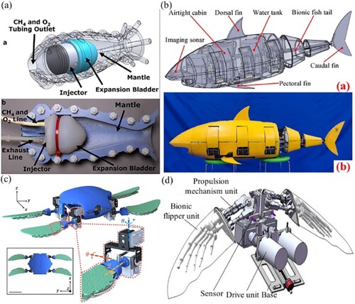
Currently, according to the different swimming mechanisms of water organisms, researchers roughly categorize underwater bionic robots into water-jet, wiggle, hydrofoil, and web-swimming methods according to their propulsion technique. Waterjet-propelled underwater bionic robots, represented by a pulse high pressure-type working mechanism, have the advantages of instantaneous motion speed and relatively sufficient power while also having the disadvantages of high energy consumption and low efficiency. Additionally, these robots are mainly bionic and use molluscs as bionic objects. For example, in 2018, inspired by the propulsion of a squid spraying water outwards from the inside of its abdominal cavity, researchers at Cornell University developed an underwater squid-imitating robot (Keithly et al., 2018), as shown in Figure 1(a). This robot employs a combustion-explosive drive through which energy is supplied to the robot via the expansion of a soft-body cavity. This enables the robot to extrude and shoot a high-velocity water current outwards from the inside to propel it to swim forward, with an instantaneous speed of up to 0.8 m/s. The swinging propulsion underwater bionic robot, which is represented by the working mechanism of the body, middle fin and tail fin swinging each other, has the advantages of high swimming efficiency and relatively stable speed manoeuvrability. However, the disadvantage is that the acceleration motion stability is relatively poor, and the robot is a bionic object that is mainly based a fish design. In 2022, inspired by the swing of a shark's tail, scholars at Harbin Engineering University (Yan et al., 2022) developed an underwater shark-like robot, as shown in Figure 1(b). A motor is used to drive energy, and the connecting rod mechanism is employed to drive the tail fin of the robot to swing left and right in the water, thus achieving forward and steering propulsion swimming. Hydrofoil and webbed swimming both utilize limb sliding flippers to slap the water surface to move forward to provide thrust. In these systems, the hydrofoil propulsion of an underwater bionic robot involves intermittent propulsion based on the force of lift, and the water propulsion efficiency is high. In addition, the main disadvantage of the forward propulsion force is that the resulting movement is relatively slow, similar to the motion exhibited by sea turtles. In 2023, researchers at Yale University in the United States (Baines et al., 2022), inspired by the movement of the limb flippers of sea turtles, developed an underwater turtle-like amphibious robot, as shown in Figure 1(c). This robot employs a motor-driven energy supply to change the stiffness of its flippers via a variable stiffness material. These flippers can be used as limbs with sufficient hardness to walk on a sandy beach or as fins with sufficient softness to realize forward gliding motion in water. The webbed swimming underwater bionic robot is a kind of intermittent propulsion robot based on resistance, and its advantages are that the propulsion force in the water is relatively large and that the movement is relatively instantaneous. Moreover, the disadvantages are that there is resistance to the backward propulsion within the recovery phase of swimming, reducing the efficiency of its propulsion, and that it is mainly based on the bionic nature of semiaquatic animals. In 2022, scholars at Tianjin University (Liu et al., 2022b), inspired by the movement of the forefins of a sea lion, designed an underwater imitation sea lion robot, as shown in Figure 1(d), that is powered by a motor-driven energy supply. Through the transmission of the swing mechanism and the crank-rocker mechanism, the robot simulates the propulsion trajectory of a sea lion and is capable of generating a large thrust peak at a higher clapping frequency.

Figure 1. Bionic underwater robot: (a) underwater squid-imitating robot (Keithly et al., 2018); (b) underwater shark-like robot (Yan et al., 2022); (c) underwater turtle-like amphibious robot (Baines et al., 2022); and (d) underwater imitation sea lion robot (Liu et al., 2022b).

Notably, the swimming style of a frog can also be described as the abovementioned webbed swimming style. However, the frog can overcome backward movement within the recovery phase of swimming by controlling the change in the size of the flipper area, making its propulsion very efficient. To date, there have been no reports on the underwater frog-like flipper mechanism, and most related works have focused on the frog-like hindlimb mechanism for jumping (Fan et al., 2022; Lu et al., 2016; Pan et al., 2023) and swimming (Gul et al., 2017; Pan et al., 2024; Shimizu et al., 2017). Therefore, the flipper mechanism is often simplified as an articulated passive rigid structure. Because frogs are small in size and light in weight and have a strong skeletal muscle structure and well-developed hind limbs, they not only have excellent jumping ability but also swim very quickly in water. Although the frog's hind limbs act as actuators to generate explosive force during movement and maintain smooth movement through the coordinated movement of all four limbs, it is difficult for a frog in water to perform strong manoeuvring and propulsion during swimming without variation in the size of the flippers between the toes. Because the frog has very high dexterity in controlling changes in the state of the flippers, its hind limbs can quickly return to their original position within a very short recovery phase, generating very little resistance to backwards propulsion within the recovery phase, which results in very efficient swimming. Therefore, the frog-like flipper mechanism is of great practical significance and research value for the development of frog-like robot technology.

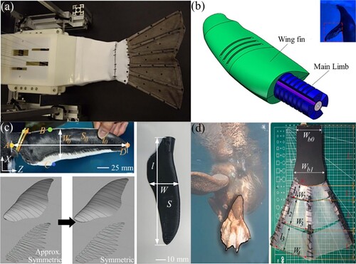
Although there are no known studies on frog flippers, there have been studies on other organisms that characterize the movement of webbed fins while swimming in water. For example, in 2012, Christopher et al. (Esposito et al., 2012) designed a fish-like tail webbing fin based on the bio-organizational movement mechanism of the strips in the tail fin of bluegill sunfish, as shown in Figure 2(a). By controlling the strips to simulate the conformation state of the tail webbing fins, at the same frequency, more flexible fins produce less peak force than stiffer fins. A fin with 500 times the stiffness produces the largest thrust force, and a fin with 1000 times the stiffness produces the largest lift force. In 2022, researchers at Shenyang University of Technology (Zhao et al., 2022) designed a pneumatic soft-type imitation sea lion front flipper fin based on the structural characteristics and propulsion mechanism of the front flipper of a sea lion, as shown in Figure 2(b). After nonlinear hydrodynamic analysis, the dynamic characteristic curve of the front flipper fin for propulsion in water was obtained, which confirmed that the soft-type front flipper fin has superior in underwater propulsion performance. In 2021, engineers in Japan (Shen et al., 2021) investigated a flexible penguin-like webbed wing based on the posture and movement characteristics of penguin wings, as shown in Figure 2(c), by adjusting the three degrees of freedom to obtain the flapping, feathering, and pitching movements needed to generate the main thrust during water movement. Thus, verifying that the pitching movement can effectively change the thrust direction, while the feathering movement can avoid stalling and increase the net thrust by 7 times. In 2021, researchers at Zhejiang University of Science and Technology (Chen et al., 2021) studied a kind of bending imitation beaver webbed foot according to the movement principle of the flexible webbed foot of a beaver, as shown in Figure 2(d). After hydrodynamic and paddling performance studies of bendable webbed feet were performed, it was verified that bendable webbed feet could more effectively reduce the resistance of webbed feet in the recovery phase than unbending webbed feet under different flow rates. Furthermore, an improved motion trajectory was also proposed, which added a pause process after the paddling propulsion phase to reduce the resistance generated by water flow and improve stroke performance. Based on the above mentioned extensive researches on bionic webbed-fins (Dong et al., 2020;  Liu et al., 2022a; Zhu and Bi, 2017), in order to solve the problems of insufficient adaptation, poor stability, and inefficient propulsion of passive flippers in water environments in the field of frog-like swimming robots. First, inspired by the structure and movement of frog flippers, in this study, the transmission design of linkage gear and the high deformation property of silicone material were used to develop a frog-like flipper mechanism that enhances underwater swimming, environmental adaptability, and the flexibility of stretching posture change. Frogs in water can be simulated by spreading flippers to expand or reduce their area of contact with water to decrease water drag and improve propulsion efficiency during swimming. Then, by combining the equations of motion and the deformation theoretical model of flippers, a fluid dynamics model of flippers in water was derived. The underwater swimming performance of the flippers was theoretically calculated and simulated via computational fluid dynamics (CFD). Finally, the results of the experiment were used to verify the rationality and correctness of the theoretical derivation of the flipper. In addition, compared to fixed, passive folding, and passive spring-loaded flippers, the proposed flippers enable the frog-like swimming robot to reduce water drag and increase propulsive force in a flowing water environment, thereby realizing the swimming characteristics of fast swimming velocity and high dexterity.

Figure 2. Underwater bionic web-fin mechanism: (a) fish-like tail webbing fin (Esposito et al., 2012); (b) imitation sea lion front flipper fin (Zhao et al., 2022); (c) penguin-like webbed wing(Shen et al., 2021); and (d) imitation beaver webbed foot(Chen et al., 2021).

2. Mechanistic design of the frog-like swimming flipper

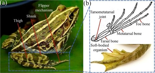
Because frogs possess a strong structural organization system of hind limbs, they can not only jump on land but also swim in water and even jump on the surface of the water. In the abovementioned explosive movements, flippers play an irreplaceable role, especially in the water, to complete swimming activities such as advancing, turning and diving. As shown in Figure 3(a), the hindlimb structural system mainly consists of a thigh, a calf and a flipper mechanism. The flipper mechanism involves a series of flexible toes comprising a tarsometatarsal joint, a tarsal bone, a metatarsal bone and a phalanx bone, and the toes are connected by soft tissue to form a similar folding fan shape, as shown in Figure 3(b).

Figure 3. Biological frog structure: (a) hind limb structure composition and (b) flipper mechanism composition.

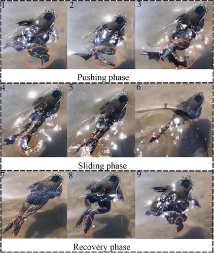
By observing the swimming process of frogs in water, we determined that the hind limbs can be approximately divided into pushing, sliding and recovering phases during the swimming process, as shown in Figure 4(1-9). In the propulsion phase (1-3), the frog's flippers are in a curled-up state from the initial moments of the propulsion phase. As the thighs and calves stretch outwards, the flippers immediately open up, changing the area in contact with the water so that the explosive force of the thighs and calves acts on the water surface to generate sufficient thrust to swim forwards. Therefore, frogs control the speed and direction of swimming by controlling the size of the opening area of their flippers. In the sliding phase (4-6), the thighs and calves remain motionless, and the frog will control the flippers to contract immediately to reduce the flipper opening surface so that the resistance to swimming forward decreases, and it is completely possible to realize that the frog controls the sliding phase for a very short time into the recovery phase. In the recovery phase (7-9), the frog's flippers remain in a contracted state, while the thighs and calves begin to curl inwards. At this time, there is little water resistance at the contact surface between the flippers and the water, so the frog can quickly control its thighs and calves to complete the curling motion. Notably, the frog can control the sliding and recovery phases in a short period, indicating that the frog can quickly and continuously swing the flippers back and forth in the water so that its efficiency and flexibility during swimming in water are very high. In addition, the soft tissues of the flippers have flexible properties. When the flippers are subjected to explosive thrusts from the thighs and calves, the soft tissues can be deformed to cushion the reactive thrusts acting on the water surface, thus adequately protecting the other organ tissues of the hindlimb.

Figure 4. Motion mechanism of frog flippers during the paddling process.

In summary, by combining the structural parameters and motion characteristics of frog hind limb flippers, a controllable soft-body extension-driven frog-like flipper mechanism was designed, and the physical mechanism involved mainly a soft-body deformation membrane, a driving mechanism, and a toe bone, as shown in Figure 5(1) I. The driving mechanism adopts a gear linkage transmission mechanism, and the components include waterproof servos, a gear shaft, bearings and a base. The base is divided into an upper base and a lower base. To reduce the friction between the gear shaft and the base, the corresponding bearing holes are designed on the base, and the rolling bearings are mounted here, as shown in Figure 5(1) A-B. The gears are divided into service gears, transmission gears, and gear shafts, where the gear shafts are divided into 2-stage gear shafts (1 and 2), 1-stage gear shafts (5 and 6), and direction-change gear shafts (3 and 4). The number of teeth of the 2-stage gear shafts is 1.5625 times that of the 1-stage gear shafts, while the number of teeth of the direction-change gear shafts is equal to that of the 1-stage gear shafts, as shown in Figure 5(1) C-D. The 2-stage gear shafts (1 and 2) are assembled at the top of the lower base and gear-mesh with each other so that relative rotation is possible. The 1-stage gear shafts (5 and 6) and the direction-change gear shafts (3 and 4) are assembled in the middle of the lower base, where the direction-change gear shafts (3 and 4) are arranged in the middle and intermesh, respectively, with the gears of the 2-stage gear shafts (2 and 1). Moreover, the gears of the 1-stage gear shafts (6 and 5) are intermeshed. This ensures that the gear shafts (5 and 6) rotate in the same direction as the gear shafts (2 and 1).

Figure 5. Frog-like flipper mechanism design: (1) structural constituent elements; (2) kinematic relationship; (3) mechanism of soft-body membrane deformation; and (4) bionic motion.

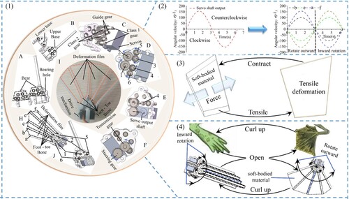
As shown in Figure 5(1) E-F, the servos are mounted at the very bottom of the lower base, and the output shaft of the servos is arranged at the back of the lower base. By installing a transmission gear on the output shaft of one end of direction-change gear shaft 4 to mesh with the gear on the output shaft of the servos, the rotation of the gear shafts (stage 1 and stage 2) is thus controlled by the rotation of the servos. As shown in Figure 5(1) J, the upper base with bearings is assembled on the front of the lower base so that its gear shafts (1–6) and servos are assembled between the upper and lower bases. As shown in Figure 5(1) H, four frog-like toe bones (a, b, e and f) were installed on the gear shaft (1-stage and 2-stage) and made to move along the axis with the gear shaft (1-stage and 2-stage). Finally, four pieces of soft deformation membranes were fixed between the toe bones. As shown in Figure 5(2), because the number of teeth of the servo gear is equal to that of the transmission gear, when the output shaft of the servo generates a periodic angular velocity, the transmission gear drives gear shaft 4 with an angular velocity equal to the output of the servo and in the opposite direction. Meanwhile, gear shaft 4 drives gear shaft 6 to rotate at equal velocity and in the same direction as the servo output so that the toe bone (a) rotates outwardly counterclockwise first and then inwardly clockwise. Since the number of teeth of the 2-stage gear shaft is 1.5625 times that of the 1-stage gear shaft, the angular velocity of gear shaft 1 is 1/1.5625th that of gear shaft 4 and is in the same direction as the servo output, so that the toe bone (b) rotates outwards counterclockwise first and then inwards clockwise. Furthermore, gear shaft 2 is driven by gear shaft 1 with equal angular velocities and in a direction opposite to the servo output so that the toe bone (e) is rotated outwardly clockwise first and then inwardly counterclockwise. Similarly, the angular velocity of gear shaft 2 is 1/1.5625th that of gear shaft 3, so the angular velocity of gear shaft 3 is equal to that of gear shaft 4 and in the opposite direction. Moreover, gear shaft 5 is driven by gear shaft 3 with the same angular velocity and in the opposite direction to the servo output so that the toe bone f rotates outwardly first clockwise and then inwardly counterclockwise. In summary, as shown in Figure 5(4), when the servo output angular velocity is counterclockwise, the toe bones (a and b) and the toe bones (e and f) rotate outwards with the symmetry axis of the toe bone c, which stretches and deforms the soft-body membrane between the toe bones (as shown in Figure 5(3)) to unfold the flippers. Similarly, when the servo output angular velocity is clockwise, the toe bones (a and b) and the toe bones (e and f) rotate inwards with the symmetry axis of the toe bone c, which shrinks and deforms the soft-body membrane between the toe bones (as shown in Figure 5(3)) and curls up their flippers.

3. Theoretical analysis of the deformation of the frog-like flipper movement

3.1. Theoretical calculation of motion

As shown in Figure 6(a), the angular velocity of the 2-stage gear shaft is 1.5625 that of the 1-stage gear shaft, and the angular velocities of the four toe bones in the flippers (a, b, e, and f) are W_a (W_t), W_b (W_t/1.5625), W_e (-W_t/1.5625), and W_f (-W_t), respectively, where W_t denotes the angular velocity of the servo output. To analyse the flipper movement regularities, constructed geometric relationships were used for derivation. First, the whole flipper mechanism was divided into left and right sides. As shown in Figure 6(b), toe bone c is made into an extension line along the direction of A₁O₁, and its length O₁A results in point A and centre point O₃ of the toe bone being in the same horizontal line, connecting point O₃. Then, toe bone b is extended by making an extension line along the direction of B₁O₂ so that it intersects with point B on line segment O₃A. Similarly, as shown in Figure 6(c), toe bone c is an extension line in the F₁O direction, the length of which is such that point F is on the same horizontal line as the centre point O₅ of toe bone f and connects with point O₅. Then, the toe bone e is extended along the direction of J₁O₄ so that it intersects line segment O₅F at point J.

Figure 6. Movement mechanism analysis of frog-like flippers: (a) overall movement; (b) left hemisphere movement; and (c) right hemisphere movement.

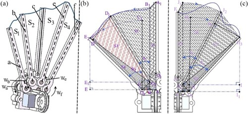
In Figure 6(b), the line segments B₁O₂ and C₁O₃ are the initial positions of the toe bone (b and a), respectively. When toe bone b is rotated by θ₁ at angular velocity W_b, the position is line segment D₁O₂. At the same time, the toe bone a rotates θ₂ with angular velocity W_a, and its position is line segment E₂O₃. At this point, the area of deformation of the soft-body membrane movement between the toe bones (c, b and a) is shown as sector E₂D₁B₁A₁AO₃ in the figure. Because the length difference between the toe bones is not large, points B₁A₁ are linked by a straight line, points B₁D₁ are connected by an arc with point O₂ as the centre of the circle, and points D₁E₂ are connected by a straight line. Therefore, the area of sector E₂D₁B₁A₁AO₃ is similar to that of polygon E₂D₁B₁A₁AO₃.

To derive the mapping relationship between the motion joint angle of the left toe bone and the motion area of the flipper, the deformed area of polygon E₂D₁B₁A₁AO₃ is divided into S1, S2, S3, S4, and ΔO₃O₂B. Here, the areas of S1 and ΔO₃O₂B are determined by the dimensions of the structure, which are fixed values, and the values are so small that they can be ignored. Thus, the motion area of the left flipper can be obtained as S_Z as follows: (1) $\begin{array}{r}{S}_Z=S_{S2}+S_{S3}+S_{S4}\end{array}$(1) The movement area of S2 is generated by the movement of toe bone b by rotating θ₁ in the centre of circle O₂, so the movement area of S2 is expressed as follows: (2) $\begin{array}{r}{S}_{S2}=\frac{{\theta }_1\pi }{{360}^{\circ }}\bullet (B_1{O}_2{)}^2\end{array}$(2) Similarly, the movement areas of S3 and S4 are generated by the movement of the toe bone a relative to the toe bone (b), so the extension line is formed along the direction AO₃, intersecting the vertically downwards extension line of point E₂ and perpendicular to point E. Furthermore, a vertical line is generated from point O₂ to line segment E₂E with respect to point E₁. The angle of ∠E₂O₃C₁ is known to be θ₂, so the angle of ∠E₂O₃E is 90°- θ₂, and the line segment E₂O₃ is the length of the toe bone (a). Therefore, the expressions for the lengths of lines E₂E and EO₃ are as follows: (3) $\begin{array}{r}\{\begin{array}{l}{L}_{E_{2}E}=\sin \left({\displaystyle \frac{\pi }{2}}-{\theta }_2\right)\ast E_2{O}_3\\ L_{E{O}_3}=\cos \left({\displaystyle \frac{\pi }{2}}-{\theta }_2\right)\ast E_2{O}_3\end{array}\end{array}$(3) It is known that the quadrangle E₂EBO₂ is a right-angle trapezoid, the upper side O₂B = O₃B = L₁, and the height is $L_{E{O}_3}+L_1$. Thus, the trapezoid change area S_T is expressed as follows: (4) $\begin{array}{r}{S}_T=\frac{\left(L_{E_{2}E}+L_1\right)\ast \left(L_{E{O}_3}+L_1\right)}{2}\end{array}$(4) Similarly, ΔE₂EO₃ is a right triangle, and the area of change in the triangle can be obtained by formula (3), whose expression is as follows: (5) $\begin{array}{r}{S}_{\mathrm{\Delta }{E}_{2}E{O}_3}=(E_2{O}_3{)}^2\ast \sin \left(2\ast \left(\frac{\pi }{2}-{\theta }_2\right)\right)/4\end{array}$(5) The area of the trapezoid S_T is composed of ΔE₂EO₃, ΔO₃BO and S4, of which ΔO₃BO is very small and negligible. The expression for the area of motion of S4 can be obtained from formulas (4) and (5): (6) $\begin{array}{r}{S}_{S4}=\frac{\begin{array}{c}2\ast \left(L_{E_{2}E}+L_1\right)\ast \left(L_{E{O}_3}+L_1\right)\\ -{\left(E_2{O}_3\right)}^2\ast \sin \left(2\ast \left(\frac{\pi }{2}-{\theta }_2\right)\right)\end{array}}{4}\end{array}$(6) To easily calculate the area S3 of ΔE₂O₂D₁, high lines are made from point D₁ to side E₂O₂, intersecting at point D. Given that the angle of ∠E₁O₂B₁ is 90 degrees, the angle change expression of ∠E₂O₂D₁ is obtained as follows: (7) $\begin{array}{r}\mathrm{\angle }{E}_2{O}_2{D}_1=\frac{\pi }{2}-\left({\theta }_1+\mathrm{\angle }{E}_1{O}_2{E}_2\right)\end{array}$(7) According to the lengths of sides E₂E₁ and E₁O₂ in the right triangle ΔE₂E₁O₂, the expression for the change in the angle ∠E₁O₂E₂ and the length of the E₂O₂ line segment can be found as follows: (8) $\begin{array}{r}\{\begin{array}{l}\mathrm{\angle }{E}_1{O}_2{E}_2=\arctan \left({\displaystyle \frac{L_{E_{2}E}-L_1}{L_{E{O}_3}+L_1}}\right)\\ L_{E_2{O}_2}=\sqrt{{\left(L_{E_{2}E}-L_1\right)}^2+{\left(L_{E{O}_3}+L_1\right)}^2}\end{array}\end{array}$(8) From formulas (8) and (7), the high line D₁D = sin (∠E₂O₂D₁) *D₁O₂ in ΔE₂O₂D₁, and the area expression of S3 can be calculated based on the triangle area formula: (9) $\begin{array}{rl}{S}_{S3}& =(\sqrt{{\left(L_{E_{2}E}-L_1\right)}^2+{\left(L_{E{O}_3}+L_1\right)}^2}\\ & \ast \sin \left(\mathrm{\angle }{E}_2{O}_2{D}_1\right)\ast D_1{O}_2)/2\end{array}$(9) By substituting formulas (2), (6) and (9) into formula (1), the area motion equation S_Z of the left flipper can be further obtained. Similarly, by substituting formulas (2-2), (6-6) and (9-9) into formula (1-1), the equation S_Y for the area motion of the right flipper can be further obtained (see Appendix 1 for details). According to the deformation motion equation of the left and right sides of the flipper, the area motion equation S_J of the whole flipper is obtained, and its expression is as follows: (10) $\begin{array}{r}{S}_J=S_{S2}+S_{S3}+S_{S4}+S_{S6}+S_{S7}+S_{S8}\end{array}$(10) As shown in Figure 6(a), the area of motion S₁ between toe bone (a) and toe bone (b) is referred to as sub-flipper 1, the area of motion S₂ between toe bone (b) and toe bone (c) is referred to as sub-flipper 2, the area of motion S₃ between toe bone (c) and toe bone (e) is referred to as sub-flipper 3, and the area of motion S₄ between toe bone (e) and toe bone (f) is referred to as sub-flipper 4. By using equation (10), the equation of motion for the area of the sub-flipper can be determined. The expression is as follows: (11) $\begin{array}{r}\{\begin{array}{l}{S}_1=S_{S3}+S_{S4}\\ S_2=S_{S2}\\ S_3=S_{S6}\\ S_4=S_{S7}+S_{S8}\end{array}\end{array}$(11) where S₁, S₂, S₃, and S₄ are mainly determined by the swing and length of toe bone (a), toe bone (b), toe bone (e), and toe bone (f), respectively.

3.2. Calculation of the deformation theory model of the soft-body membrane

The material of the sub-flipper in the frog-like flipper mechanism is silicone, which is a superelastic material that can undergo large deformations under the action of external forces. Moreover, there is a high degree of nonlinearity between the strain and stress of the material. By using the Nrd-order Ogden constitutive model, the static deformation response of soft materials under external forces can be accurately predicted. According to the stress–strain theory, it is assumed that the silicone material is isotropic and incompressible, and its strain energy function is expressed as follows: (12) $\begin{array}{r}\{\begin{array}{l}W\left(E\right)=W\left(I_1,I_2,I_3\right)\\ I_1={\lambda }_1^2+{\lambda }_2^2+{\lambda }_3^2\\ I_2=({\lambda }_1{\lambda }_2{)}^2+({\lambda }_2{\lambda }_3{)}^2+({\lambda }_1{\lambda }_3{)}^2\\ I_3=({\lambda }_1{\lambda }_2{\lambda }_3{)}^2\end{array}\end{array}$(12) Where I₁, I₂, and I₃ are the three invariants of the strain tensor, which are the axial, circumferential, and radial principal elongation ratios of the sub-flipper, respectively. Based on formula (12), Ogden's model with main elongations λ₁, λ₂, and λ₃ in three directions can be expressed as independent variables as follows: (13) $\begin{array}{r}W=\sum _{c=1}^N\frac{{\mu }_c}{{\alpha }_c}\left({\lambda }_1^{{\alpha }_c}+{\lambda }_2^{{\alpha }_c}+{\lambda }_3^{{\alpha }_c}-3\right)+\sum _{k=1}^N\frac{1}{D_k}(J-1{)}^{2k}\end{array}$(13) Where N is the order of the Ogden model (N = 3); μ_c与 α_c (c = 1,2,3 … . N) are the model parameters; and D_k (c = 1,2,3) is an incompressible parameter of the material. Thus, J = λ₁λ₂λ₃= 1 is valid. To account for the correspondence between the model and linear Hooke's law in the case of small deformations, the initial shear modulus (μ) of the material of this sub-flipper and the model parameters (μ_c and _αc) must satisfy $2\mu =\sum _{c=1}^3{\mu }_c{\alpha }_c$. Combined with formula (13), according to the Ogden hyperelastic principal configuration under incompressible conditions, the expression of the variable energy density function at this point is as follows: (14) $\begin{array}{r}{W}_N=\sum _{c=1}^N\frac{{\mu }_c}{{\alpha }_c}\left({\lambda }_1^{{\alpha }_c}+{\lambda }_2^{{\alpha }_c}+{\lambda }_3^{{\alpha }_c}-3\right)c=1,2,\dots .,N\end{array}$(14) Then, according to formulas (12) and (14), through the Piola–Kirchhoff stress and Cauchy–Green strain relationships, the expression of the relationship between the principal stress and principal tensile rate can be obtained as follows: (15) $\begin{array}{r}{\sigma }_N=\sum _{c=1}^N{\mu }_c{\lambda }_j^{{\alpha }_c}+\rho c=1,2,\dots .,N\end{array}$(15) Where p is the hydrostatic pressure. For the case of uniaxial stretching of the sub-flipper, it is assumed that the tensile direction is 1 and that the tensile rate is λ₁. Then, the corresponding stress state is σ1 = σ2 = σ3 = 0, and the hydrostatic pressure is p = σ2 = σ3 = 0. When λ₁λ₂λ₃ = 1, ${\lambda }_2={\lambda }_3=1/\sqrt{{\lambda }_1}$ can be introduced. By substituting the above correlation values into formula (15), the mapping relationship between the uniaxial tensile principal stress and tensile strength of the Nrd-order Ogden model can be further obtained, and the expression is as follows: (16) $\begin{array}{r}{\sigma }_N=\sum _{c=1}^N{\mu }_c\left({{\lambda }_1}^{{\alpha }_c}-{{\lambda }_1}^{-\frac{1}{2}{\alpha }_c}\right)c=1,2,\dots .,N\end{array}$(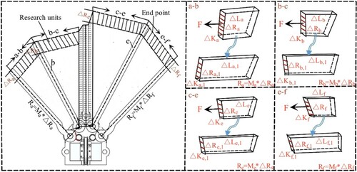16) As shown in Figure 7, from the end of each sub-flipper downwards, an approximate quadrilateral cube with an initial width of ΔR_i is intercepted, with an initial length of ΔL_i and an initial thickness of ΔK_i in its natural state, and the sub-flippers of this approximate quadrilateral cube are referred to as the research unit. After the tensile movement of the four toe bones i, the research unit will produce a certain approximate uniaxial tensile deformation, and its length, thickness, and width become ΔL_i,1, ΔK_i,1, and ΔR_i,1, respectively. (where i represents four different toe bones, a, b, e, f; and R_i is the length of the toe bone) (17) $\begin{array}{r}\{\begin{array}{l}{\lambda }_1={\displaystyle \frac{\mathrm{\Delta }{L}_{i,1}}{\mathrm{\Delta }{L}_i}}\\ {\lambda }_2={\displaystyle \frac{\mathrm{\Delta }{K}_{i,1}}{\mathrm{\Delta }{K}_i}}={\displaystyle \frac{1}{\sqrt{{\lambda }_1}}}\\ {\lambda }_3={\displaystyle \frac{\mathrm{\Delta }{R}_{i,1}}{\mathrm{\Delta }{R}_i}}={\displaystyle \frac{1}{\sqrt{{\lambda }_1}}}\end{array}i=a,b,e,f\end{array}$(17) From formula (17), after tension, the length, thickness, and width of the research unit become ΔL_i1 = ΔL_i*λ₁, $\mathrm{\Delta }{K}_{i1}=\mathrm{\Delta }{K}_i/\sqrt{{\lambda }_1}$, and $\mathrm{\Delta }{R}_{i1}=\mathrm{\Delta }{R}_i/\sqrt{{\lambda }_1}$, respectively. Based on the N-order Ogden model mechanism formula (16), the relationship between the tensile force and the tensile rate of the research unit in the sub-flipper can be further deduced with the following expression: (18) $\begin{array}{r}{F}_i={\sigma }_N\left({\lambda }_1\right)\ast \left(\mathrm{\Delta }{R}_{i,1}\ast \mathrm{\Delta }{K}_{i,1}\right)i=a,b,e,f\end{array}$(18) Where $\mathrm{\Delta }{R}_{i,1}\ast \mathrm{\Delta }{K}_{i,1}$ is the cross-sectional area of the research unit after tension and ${\sigma }_N\left({\lambda }_1\right)$ is the Cauchy stress over the cross-sectional area. By substituting Equations (16) and (17) into Equation (18), the force–displacement deformation equations of the sub-flipper under stretching between the toe bones (i) can be calculated as follows: (19) $\begin{array}{rl}{F}_i& =\sum _1^{M_i}[\mathrm{\Delta }{R}_i\ast \mathrm{\Delta }{K}_i\ast (\sum _{c=1}^{\text{N}}{\mu }_c[{\left(\frac{\mathrm{\Delta }{L}_{i,1}}{\mathrm{\Delta }{L}_i}\right)}^{{\alpha }_c-1}\\ & \ast \left(1-{\left(\frac{\mathrm{\Delta }{L}_{i,1}}{\mathrm{\Delta }{L}_i}\right)}^{-\frac{3}{2}{\alpha }_c}\right)])]i=a,b,e,f\end{array}$(19) The higher the order of the Ogden model in Equation (19) is, the greater its fitting accuracy to the experimental data. Therefore, the value of (N) in this paper is taken to be 3. When N = 3, then α₁ = α₂ = α₃ = 2. In this paper, the sub-flippers are made of silicone, and their shear modulus is μ₁ = μ₂ = μ₃= 0.45. M_i is the number of research units intercepted from the end of toe bone (i) downwards in the sub-flipper, that is, M_i = R_i/ΔR_i. The larger its value is, the smaller the initial width and the more accurately the value of (F_i) is obtained. According to the geometrical relations of the area movement theory in Subsection 3.1, during the deformation movement of the sub-flipper, ΔL_i,1 is approximately equal to the mutual movement distance between the ends of the toe bones, which is ΔL_a,1≈E₂D₁, ΔL_b,1≈D₁B₁, ΔL_e,1≈B₁J₂, and ΔL_f,1≈J₂H₁. (20) $\begin{array}{r}\{\begin{array}{l}{E}_2{D}_1=\sqrt{\begin{array}{l}{\left(L_{E_2{O}_2}\right)}^2+{\left(R_b\right)}^2-2\\ \ast L_{E_2{O}_2}\ast R_b\cos \mathrm{\angle }{E}_2{O}_2{D}_1\end{array}}-\mathrm{\Delta }{L}_a\\ D_1{B}_1=2\ast R_b\ast \sin \left(\frac{{\theta }_1}{2}\right)-\mathrm{\Delta }{L}_b\\ B_1{J}_2=2\ast R_e\ast \sin \left(\frac{{\theta }_3}{2}\right)-\mathrm{\Delta }{L}_e\\ J_2{H}_1=\sqrt{\begin{array}{l}{\left(L_{H_3{O}_4}\right)}^2+{\left(R_e\right)}^2-2\\ \ast L_{H_3{O}_4}\ast R_e\cos \mathrm{\angle }{H}_3{O}_4{J}_2\end{array}}-\mathrm{\Delta }{L}_f\end{array}\end{array}$(20) Where R_i is the length of the toe bone (i represents four different toe bones, taking the values a, b, e, f); E₂D₁, D₁B₁, B₁J₂, and J₂H₁ are derived from the edge and angle relationship equations of ΔE₂O₂D₁, ΔD₁O₂B, ΔJ₁O₁J₂, and ΔJ₂O₁H₃ in Figure 6(a-c), respectively.

Figure 7. Tensile principle diagram of the soft-body deformation membrane in frog-like flippers Assuming that the tensile rate in the length direction is λ₁, it follows from the deformation theory:

4. Theoretical analysis of frog-like flipper hydrodynamics

As shown in Figure 8(a), according to the characteristics of the frog's flippers swimming in the water, the frog-like flippers are spread between the pushing phase and the sliding phase, and closed between the sliding phase and the recovery phase. Therefore, the flippers divide the water flow field into incident flow zone and static flow zone during the above process, as shown in Figure 8(b–d). When the frog is in the pushing phase, the flippers are based on the outward movement of the hind limbs, which are paddling forward by spreading the flippers, at which time the water flow strikes the front of the flippers and creates a hydrodynamic resistance (indicated by the light blue arrows in Figure 8(b)).when the flippers paddle backward, it will drive the water flow behind the flippers so that the speed of the water flow behind it becomes greater relative to the water flow in front of it, a part of the water flow behind it will flow forward, a part of the water flow will flow from the bottom and the two side surfaces of the flippers to the front, and it will form a counter-current zone. At the same time, the water flow behind the flippers creates an opposing force to the back of the flippers, which causes the flippers to create a thrust to swim forward (indicated by the red arrow in Figure 8(b)). When the frog is in the recovery phase, based on the inward movement of the hind limbs, when the flippers paddle forward, the front water flow will be blocked and driven by the flippers so that the velocity of the water flow in the back of the flippers will decrease relative to the front water flow, and a small part of the water flow will flow from the bottom and both sides of the flippers to the back of the flippers, at which time a return zone is formed in the back of the flippers. At the same time, the water flow in front of the flippers creates an opposing force to the front of the flippers, which causes the flippers to generate backward fluid drag, as shown in Figure 8(c). However, frogs reduce their area of contact with water by closing their flippers, allowing the flippers to reduce water resistance during the recovery phase.

Figure 8. Changing state of water flow field during paddling with frog-like flippers:(a) flipper movement state;(b) changes in the water flow field during the propulsion phase;(c) changes in the water flow field during the recovery phase.

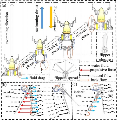
According to the above analysis of the movement of the frog's flipper in water, the hydrodynamics of the flipper are affected mainly by the coefficient of fluid drag, the frontal contact area and the fluid velocity. The force generated by the incident water flow is defined as the fluid drag (F_d) of the flippers as they paddle in the water. The back of the flippers interacts with the water flow to create a forward reaction force called paddling propulsion (F_M). The flippers studied in the paper oscillated in the horizontal plane, and the width of the flippers on the side of the vertical horizontal plane was very small (small area), so the fluid lift (F_L) on the side of the flippers during paddling was small and negligible. Considering the state in which the flippers produce forward motion in paddling, combined with the hydrodynamic calculation method, the hydrodynamic solution formula for the flippers is established, and the expression is as follows: (21) $\begin{array}{r}\{\begin{array}{l}{F}_d=C_D\ast {\rho }_S\ast \left(S\ast \sin \left(\gamma \right)\right)\ast U_W|U_W|\bullet \hat{X}\\ F_M=C_D\ast {\rho }_S\ast \left(S\ast \sin \left(\gamma \right)\right)\ast U_M|U_M|\end{array}\end{array}$(21) Where ρ_S is the density of flowing water, which is 1.0 × 10³ kg-m-3; S denotes the effective area of the flippers in contact with the water flow during paddling, and its value is S_J in Equation (10); γ is the angle between the water flow and the mutual contact area of the flipper surface, whose flippers rotate in the horizontal plane at an angle ranging from [0° to 180°]; and C_D denotes the coefficient of water drag in paddling, which is determined by the Reynolds number R_n for planar translation and rotation in the water flow, where R_n can be expressed in laminar and turbulent layers as follows:. (22) $\begin{array}{r}{R}_n=\frac{{\rho }_S\ast |U|\ast D}{\varsigma }\end{array}$(22) Where D is the characteristic length along the direction of the water flow velocity, which is the maximum width of the flippers (140 mm), and ζ is the dynamic viscosity of the water fluid, which is 1.01×10⁻³ Pa⋅s when the water fluid velocity is less than 1 m/s. The above parameters are substituted into Equation (22) to obtain the Reynolds number, which is less than 2*10⁵. Then, the water drag coefficient is 1.

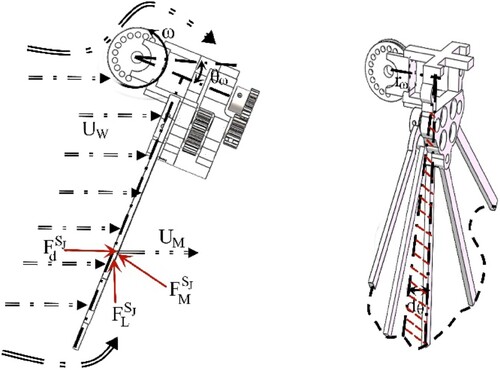
From Equation (21), where U_W represents the integrated velocity of the linear velocity U_M of the paddling swing in the flippers and the velocity of the water fluid V_a, its expression is as follows: (23) $\begin{array}{r}\{\begin{array}{l}{U}_W=\{\begin{array}{ll}{V}_a-U_M,& V_a\ge U_M\\ 0& V_a<U_M\end{array}\\ U_M=\omega \times r_{\omega }\end{array}\end{array}$(23) Where ω and r_ω denote the angular velocity of the flipper rotation and the corresponding radius of rotation, respectively, as shown in Figure 9. When the frog is paddling, the area of the flipper opening is controlled to regulate the water drag and water propulsion during the propulsion, sliding, and recovery phases. According to the theory of flipper deformation in Subsection 3.1, the mapping relationship between the flipper area and the output angle of the frog-like flippers is known, and by substituting formula (10) into formula (21), the hydrodynamic equations of the flippers are obtained by using the integral method of derivation. The expression is as follows: (24) $\begin{array}{r}\{\begin{array}{l}{F}_d=\underset{0}{\overset{S_J}{\int }}{C}_D\ast {\rho }_S\ast U_W|U_W|\mathrm{d\theta }\bullet \hat{X}\\ F_M=\underset{0}{\overset{S_J}{\int }}{C}_D\ast {\rho }_S\ast U_M|U_M|\mathrm{d\theta }\end{array}\end{array}$(24) Where S_J is the total area of the flippers, and its value varies with the size of the sub-flipper spreading angle, whose mapping relationship is given by Equation (10), where the input angle θ ranges from [0°, 90°].

Figure 9. Hydrodynamic force state of frog-like flippers.

5. Calculations and research based on structural parameters

5.1. Calculation analysis of the motion and deformation of frog-like flippers

Due to the limitation of the overall size of the frog-like swimming robot, the fixation parameters of its flipper mechanism mainly depend on the lengths R_i (a, b, e, and f) of the four toe bones, that is, 65, 70, 85, and 77 mm, and the value of the fixed toe bone c is taken as 67 mm. By using the equations of motion (11-12) for the area of the flippers in subsection 3.1 and equation (20) for the distance of motion between the ends of toe bone (i), the angle of motion of its flippers depends on the angular velocity (W_t) input from the servo. After the theoretical calculation by Matlab software, the influence characteristic curve of the flipper output is shown in Figure 10(a–c), where W_t is set to control the servo output angle as [0°, 90°].

Figure 10. Influence characteristic curves of the frog-like flipper output: (a) variation in the spreading area; (b) variation in the spreading angle; (c) variation in the distance between toe bones(i); and (d) prototype measurement experiments

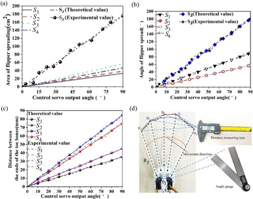
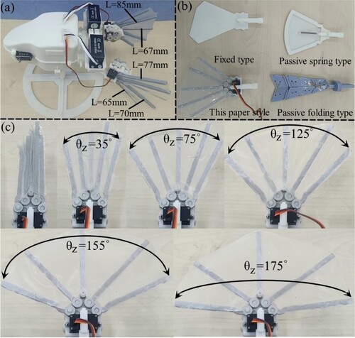
Figure 10(a–c) shows that the total area and angle of the flippers spread, the area and angle of the sub-flippers spread, and the distance between the toe bone(i) end in the sub-flippers increases with increasing angle of the servo output, showing a positive proportional relationship. Additionally, the larger the angle of its output is, the larger the value of its influence characteristic. When the servo output is 90 degrees, the total flipper opening area is close to 180 cm² and the total flipper spreading angle reaches 180 degrees. Figure 10(a) shows that when the servo outputs a certain angle, each of its sub-flippers has a different area, and the order of its area from the largest to the smallest is as follows: sub-flipper 3 is the largest, followed by sub-flipper 4; sub-flipper 2 is ranked third, and the smallest is sub-flipper 1. Similarly, as shown in Figure 10(c), the size of the distance moved by the end of the toe bones in each of its sub-flippers is the same as the regularity of the spreading area. However, as shown in Figure 10(b), the angle of spreading of sub-flipper 1 is the same as that of sub-flipper 4, sub-flipper 3 is the same as that of sub-flipper 2, and the angle of spreading of sub-flippers 1 and 4 is greater than those of sub-flippers 2 and 3. It can be concluded that when the angle of spreading of the sub-flippers is the same, the area of spreading of their sub-flippers and the distance of movement between the ends of the toe bones are also related to the length of the toe bones. In the geometric relationship of the sub-flipper, it is known that sub-flippers 1, 2, 3, and 4 are subjected to the corresponding tensile movement of the toe bones (R_a, R_b, R_e, and R_f), respectively, and the toe bone length relationship is R_e > R_f > R_b > R_a. Therefore, when the angle of spreading of the sub-flipper is the same, the area of spreading of its sub-flipper and the distance between the ends of the toe bones are positively related to the length of the toe bones. Moreover, the greater the lengths of the toe bones are, the greater the area of spreading of the sub-flipper, and the greater the corresponding distance of movement between the ends of the toe bones. To verify the correctness of the above theoretical derivation of the flippers, relevant prototype measurement experiments were performed, as shown in Figure 10(d). When the control servo outputs a certain angle, the total angle (θ_J) of the flipper spread is measured with a protractor, and the approximate flipper spread sector area is then obtained by rotating the angle (θ_J) with the centre of the circle O_S. By measuring the radius as R_J, the area of the sector in which the flippers are spread was calculated. Moreover, the distance between the ends of the toe bones (i) were measured with a distance measuring tape, and these experimental data are plotted in Figure 10(a-c). The experimental values coincide with the theoretical value, but there is a certain small error. Therefore, it shows that the theoretical derivation has a certain correctness.

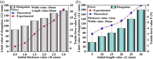
The sub-flipper between the toe bones (i) is made of a large deformation silicone elastic material, so the sub-flipper material must conform to the deformation theoretical model of Equation (20) in addition to fulfilling the area motion mechanism described above. To first determine the correctness of this theoretical derivation, relevant validation tests were carried out (see Appendix 2). The data from the experimental tests (initial thickness ΔK, initial length ΔL, elongation limit (ΔLL), and tensile force (F)) are plotted in Figure 11(a,b). Figure 11(a) shows that the elongation limit (ΔLL) of the sub-flipper is approximately proportional to the initial thickness (ΔK). The larger the initial thickness is, the larger the elongation limit is. Similarly, as shown in Figure 11(b), the elongation limit value (ΔLL) of the sub-flipper also shows an approximately proportional relationship with the initial length (ΔL), and the larger the initial length is, the larger its elongation limit value is. Compared to Figure 11(a), from the range values of the experimental values of tensile force (dotted line with red spheres), for approximately the same limiting value of elongation (ΔLL), increasing the initial thickness requires much more tensile force to be overcome than increasing the initial length. Therefore, the initial thickness of the sub-flipper material is selected to be small, while the initial length is selected to be longer to achieve a larger elongation with a relatively small tensile force. The above experimental test data (initial length, initial width, and initial thickness) were then brought into the force–displacement deformation equation, Equation (20), to determine the theoretical value of the tensile force of the sub-flipper material, as indicated by the dotted line with the blue sphere in Figure 11(a,b). The theoretical values coincide with the experimental values, but there is a small error, thus showing that the theoretical derivation of the deformation theory about the material of the sub-flipper has a certain correctness.

Figure 11. Experimental tests of the tensile deformation of the material of the sub-flipper: (a) Mechanical properties of the effect of the initial thickness on the elongation limit. (b) Mechanical properties of the effect of the initial length on the elongation limit.

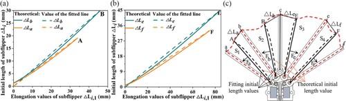
To ensure that the flipper mechanism can unfold the four sub-flippers through the servo handle with the maximum output torque, the sub-flippers should also have a certain degree of toughness. Therefore, a suitable thickness, width and length of the sub-flippers should be obtained. The detailed procedure is shown in Appendix 3, where the parameter values of Equation (A-3), Equation (A-4), and (A-5) in the Appendix are brought into Equation (20), and the initial length (ΔL_i) at the end of the sub-flipper is obtained by using MATLAB. It varies with the value of elongation (ΔL_i,1), as shown in the solid curve in Figure 12(a,b). The dark cyan solid lines in Figure 12(a,b) are the initial length value change curves of sub-flipper 2 and sub-flipper 3, respectively, while the orange solid lines are the initial length value change curves of sub-flipper 1 and sub-flipper 4, respectively. From the figure, it can be seen that as the elongation of the sub-flipper increases, its initial value length increases, but the theoretical value curve shows a miniature arc change, which will be put into the flipper mechanism, as shown by the black dotted line in Figure 12(c). Considering that in the process of making sub-flippers, it will be more difficult to cut and fix the treatment according to the theoretical initial value curve. To address the above problem, we fit the line with an initial length by connecting the maximum point (A, B, E, and F) of the initial value curve of the theoretical values with the origin in Figure 12(a,b), and this line shows a positive relationship. It has a very small error from the theoretical curve value, as shown by the dashed line in Figure 12(a,b) and the solid black line in Figure 12(c).

Figure 12. Optimization analysis of the initial lengths of the sub-flippers: (a) initial lengths of sub-flipper 1 and sub-flipper 2; (b) initial lengths of sub-flipper 3 and sub-flipper 4; and (c) representation of the initial lengths in the flipper mechanism.

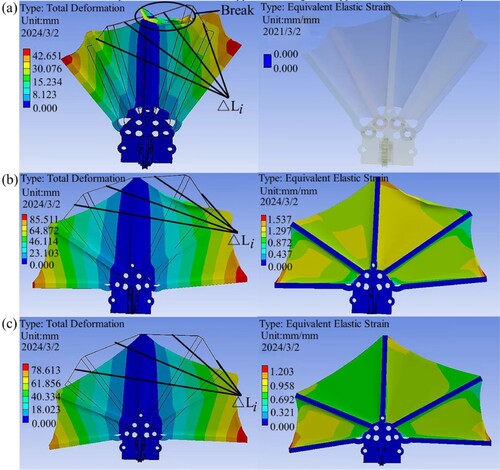
To verify the effect of the above optimized values of the fitted initial length on the mechanical properties of the sub-flippers during deformation, we used SolidWorks software to construct a 3D model based on the toe bone length (R_i) parameter, the thickness (1 mm) of the flipper, and the fitted initial length. We also built two 3D models whose initial lengths were different from the fitted initial lengths. That is, one was smaller than the fitted initial length, and the other was larger than the fitted initial length. Then, the above three models were imported into Ansys software, the material of the model in the software was set to silicone, and the driving torque was set to the same maximum torque as the servo output. The results of the simulation calculations and processing are shown in Figure 13(a–c). The solid boxed line models in Figure 13(a–c) show the three models mentioned above. From the initial value length of the sub-flippers in the modelling, the initial length is the smallest in Figure 13(a), while the initial length is the largest in Figure 13(c). Therefore, Figure 13(b) shows the optimized fitted initial length. As seen from the legend values of the left deformation results in Figure 13(a–c), the amount of sub-flipper deformation gradually increases with the change in colour from both bottom to the top. As shown in Figure 13(a), the sub-flippers have a limiting destructive failure at a deformation amount of approximately 42 mm, resulting in a deformation failure as well as an equivalent elastic strain value of 0, which makes the flippers unfold at a relatively small angle. A comparison of Figure 13(a,b) shows that the deformation in Figure 13(b) is not only larger than that in Figure 13(a) but also that the flipper spreading angle can reach 180 degrees, which is in line with the theoretical value of the spreading angle in Figure 10(b). Therefore, the initial length of the sub-flipper is selected to be too small, which will result in the sub-flipper breaking down during the unfolding of the flippers and not being able to unfold to a greater angle. Similarly, a comparison of Figure 13(c,b) shows that the flipper spreading angle in Figure 13(c) can also reach 180 degrees, but the amount of deformation and equivalent elastic strain in the figure are smaller than those in Figure 13(b). Therefore, if the initial length of the sub-flipper is too large, the toughness of the sub-flipper during unfolding will relatively decrease, and the sub-flipper will be more susceptible to deformation by external forces . In summary, under a certain thickness, width, and torque of the sub-flipper, by optimizing the initial length through the force–deformation equation, the mechanical kinematic performance of the sub-flipper in the frog-like flipper mechanism can be improved.

Figure 13. Simulation calculations of the flipper based on ANSYS software: (a) initial length of the sub-flipper is less than the value of the fitted initial length curve; (b) initial length of the sub-flipper is equal to the value of the fitted initial length curve; and (c) initial length of the sub-flipper is greater than the value of the fitted initial length curve.

5.2. Calculated hydrodynamic analysis of frog-like flippers

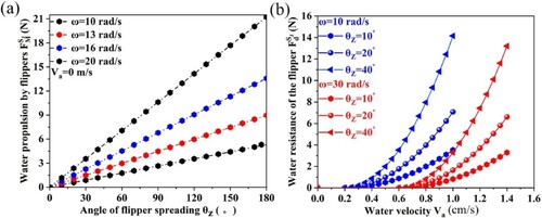
In addition to verifying the theoretical model of flipper movement and deformation mentioned in section 5.1 above, it is also necessary to qualitatively determine the hydrodynamic performance characteristics of the frog-like flipper in water. By implementing formula (24) into MATLAB software for calculation and simulation, the data on the water propulsion and water drag of the flipper mechanism were obtained, as shown in Figure 14(a–d). Figure 14(a) shows that when the water velocity (V_a) is 0, the propulsion force of the flipper paddling in water is proportional to the angle at which the flipper spreads and reaches the maximum value at 180°. Moreover, the propulsion force is proportional to the velocity of the swing of the flippers. The faster the swing is, the greater the propulsion in water. As shown in Figure 14(b), the flippers swing at an angular velocity of 10 rad/s, and their linear velocity is 0.2 cm/s. When the water velocity is within [0,0.2 cm/s], the water drag on the flippers is 0. When the water velocity is greater than 0.2 m/s, the water drag on the flippers is parabolically proportional to the water velocity, and the greater the water velocity is, the greater the water drag. Furthermore, the water drag is also directly proportional to the angle of flipper spread; the greater the angle of flipper spread is, the greater the drag value. Similarly, when the angular velocity of the flipper swing is increased to 30 rad/s and its linear velocity (0.6 cm/s) is greater than the water velocity (0.2cm/s), the flipper is subjected to 0 water drag at a water velocity of [0,0.6 cm/s], and the flipper produces water drag when the water velocity is greater than 0.6 cm/s. Therefore, when the water flow velocity is less than the linear velocity of the flipper swing, there is no water drag on the flipper; in contrast, the flipper is subjected to water drag during the swing. When the water velocity increases, in addition to reducing the flipper spreading area, the water drag can be resisted by increasing the swinging velocity of the flipper.

Figure 14. Theoretically calculated values of the flipper hydrodynamics: (a) water propulsion based on the flippers and (b) water resistance based on the flippers.

To verify the correctness of the above theoretical numerical results, the model of the flipper mechanism was imported into the fluent module of ANSYS software, from which the hydrodynamic forces of the flipper were calculated. The sliding mesh method and dynamic mesh technique were used to simulate the motion of the flipper mechanism, and the mesh distribution of the simulation model is shown in Figure 15(a). By setting the k-ϵ turbulence model, the inlet water velocity (V_a) is 0.25 cm/s, the angular velocity of the flipper swing is 10 rad/s, and the angles of the flipper spread are 20, 60, 140 and 180 degrees. The simulation results are shown in figure A2 in appendix 4. Moreover, the linear velocity (U_M) of the swinging flipper was set to 0.9 cm/s, the flipper spreading angle (θ_Z) was set to 100 degrees, and the inlet water velocity was set to 0.1, 0.3, 0.6, 0.9, 1.2, and 1.4 cm/s. The simulation results are shown in figure A3 in Appendix 4. Due to the high density of the water flow field lines in the simulation calculation, the colour point variation overlap is high and affects the differences in the content of the pictures. Therefore, to visualize the comparison of the results, the symmetric two-point variation data on the front and back sides of the flippers were extracted from the simulation results (point F for the front side; point B for the back side) and plotted, as shown in Figure 15(b–c).

Figure 15. Simulation calculations on the flippers in the Fluent module: (a) mesh delineation of the flipper model; (b) hydrodynamic simulation analysis based on the spreading angle of the flippers; and (c) hydrodynamic simulation analysis of the flippers under the change in inlet water flow velocity.

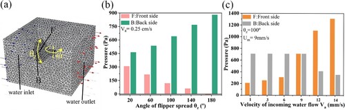
Figure 15(b) shows that the water pressure in front of the flippers is always lower than that on the back under a swinging angular velocity of 10 rad/s, and the water pressure in front of the flippers decreases as the flipper spreading angle increases, whereas that in the back shows the opposite trend. Thus, as the flippers are spread out over a larger area in the water, the pressure on the back of the flippers due to the water reaction increases, and the reaction propulsive force generated on this surface increases, thus increasing the propulsive power of the frog-like swimming robot in swimming in the water. Figure 15(c) shows that when the velocity of the inlet water flow (V_a) is less than the linear velocity of the flipper swing (U_m), the pressure at the back of the flipper will always be greater than that at the front. However, as the velocity of the inlet water flow increases, the pressure on the back of the flippers hardly changes, while the pressure on the front of the flippers gradually increases, always converging to the pressure on the back of the flippers. When the velocity of the inlet water flow (V_a) is equal to the linear velocity of the flipper swing (U_m), the pressure in front of the flipper is equal to that at the back of the flipper. It follows that when the linear velocity of the flipper in the water is greater than the velocity of the inlet water flow (V_a), the forward water reaction force on the back of the flipper in the water is always greater than the backward water reaction force on the front of the flipper, and it dominates the force generation. Thus, it is possible to use flippers to generate forward propulsion. Compared to the inlet water flow velocity, the greater the linear velocity of the flipper swing, the less backward the water reaction force applied to the front of the flipper, allowing the flipper to generate more propulsive force forward. Similarly, when the velocity of the inlet water flow (V_a) is greater than the linear velocity of the flipper swing (U_m), the pressure at the front of the flipper exceeds the pressure at the back of the flipper and increases with increasing inlet water flow velocity, whereas the pressure at the back of the flipper decreases with increasing inlet water flow velocity. It follows that the backward water reaction force in the water on the front of the flippers is always greater than the forward water reaction force on the back of the flippers, which dominates the force generation. Therefore, it is possible to use flippers to experience backward water drag. Compared to the linear velocity of the flipper swing, the greater the velocity of the inlet water flow is, the greater the backward water reaction forces on the front and back of the flippers, causing the flippers to create more water drag forward. In summary, the hydrodynamic properties of the flippers in the water in the simulation results coincide with the regular trend of the above hydrodynamic theoretical values, thus indirectly proving the correctness of the hydrodynamic model of the flippers.

6. Experimental evaluation

Based on the theoretical and simulation analysis of the above structural parameter model, the influence of frog-like flippers on the swimming performance of frog-like swimming robots was further tested through the establishment of a relevant experimental platform, and the feasibility and practicability of the structure were verified. As shown in Figure 16(a), the developed controllable soft-body extension-driven flippers were assembled on a frog-like swimming robotic platform. The flipper mechanism has four toe bones, and the toe bones are linked by a soft-body deformation membrane. The maximum area of flipper spreading is close to 180 cm², and the flipper spreading state is shown in Figure 16(c) for different driving angles. According to the revelation of frog swimming flippers, the existing flipper structures, as shown in Figure 16(b), can be approximately categorized into fixed, passive spring, and passive folding types (Wang et al., 2024). Their common feature cannot actively control the size of the flipper spreading area, especially for the fixed-type category. The passive spring and passive folding structures depend on the drag of the water flow to overcome the tensile spring tension and folding force between opposing surfaces and to control the ability of the flipper surface to work in the water; otherwise, the process will not work.

Figure 16. Testing experimental platform: (a) test prototype of the effect of flippers on the swimming performance of a frog-like swimming robot; (b) different flipper structures inspired by the swimming flippers of a frog; and (c) different angles of the spreading of the frog-like flippers.

6.1. Swimming adaptive performance tests in static water

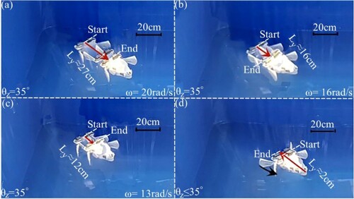
According to the three swimming phases of propulsion, sliding and recovery in water, the flippers can complete the three states of opening, holding and curling. Frog-inspired flippers are driven by remotely controlled drive motors to realize the frog-like swimming effect of the robot. After processing the experimental videos (see Video 1), the swimming sequence diagrams of the robot subjected to the variation factors of the flippers are obtained. Among them, the swimming sequence diagrams of the robot at a flipper spreading angle of 35°are shown in Figure 17(a–d). (In the figure, the "Start" mark is the start position of the robot, and the "End" mark is the end position of the robot.)

Figure 17. Swimming sequence diagram of the robot with the flippers spread at an angle of 35°: (a) motion of the robot's flippers during three stages in water; (b) angular velocity of the flippers swinging on both the right and left sides of 20 rad/s; (c) angular velocity of the flippers swinging on both the right and left sides of 16 rad/s; and (d) angular velocity of the flippers swinging on both the right and left sides of 13 rad/s.

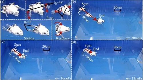
As shown in Figure 17(a), when the robot is in the water push phase, the spreading angle of the flippers on both sides is momentarily spread to 35°, and the swinging swimming under the angular velocity of the flippers on both sides is then ω. When entering the sliding phase, the spreading angle of the flippers on both sides is immediately closed, and after sliding for a period, the flippers return to their initial state during the recovery phase. Figure 17(b,d) shows that the robot is under a spreading angle of 35° on both sides of the flippers, and an experimental test is performed to study the realization of the swimming distance when the angular velocity of the swinging flipper is different on both sides. Similarly, in the case of the same angular velocity of both flippers, to further investigate the effects of different spreading angles of both flippers on the swimming distance and turning angle of the robot, the experimental results are shown in figures A4, A5, and A6 in Appendix 5. To visualize the regularity of the above experimental results, the experimental data of the robot swimming distance and the turning experiments were plotted, as shown in Figure 18(a,b).

Figure 18. Experimental tests on the swimming performance of the robot based on the flipper mechanism of this paper: (a) forward swimming distance test and (b) swimming test for turning angle.

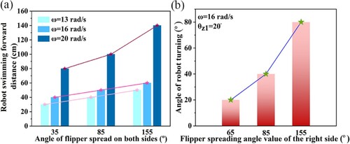
Figure 18(a) shows that when the spreading angle of the flippers on both sides is the same, as the angular velocity of the swinging flippers increases, the distance that the robot swims forward increases. Meanwhile, under the swing of the same angular velocity of the flippers on both sides, the larger the spreading angle of the flippers is, the farther the robot swam forward. In particular, when the angular velocity of the flippers is 20 rad/s, the flippers are spread at an angle of 155 degrees to drive the robot to reach a swimming distance of 140 cm. Therefore, the greater the velocity of the flipper swing and the area of the flipper in contact with the water are, the greater the forward propulsive force obtained by the flipper in the water. Similarly, as shown in Figure 18(b), the spreading angle of the right flipper (θ_z2) is larger than that of the left side (θ_z1), which causes the robot to swim in turn to the left side. Moreover, under the same velocity of swinging flippers on both sides, the greater the angle of spreading of the right flipper is, the greater the angle of turning to the left side of the swim. In summary, the robot achieves the propulsive force in the water through the flipper spreading angle and swinging angular velocity, and their relationship is consistent with the positive trend between the simulation analysis and the theoretical values. Thus, this indirectly verifies that the movement performance of this paper's flipper mechanism in static water has some reference value.

6.2. Swimming adaptive performance test compared to other types of flippers in static water

Compared to other types of flippers inspired by frogs, the flippers investigated in this paper have greater advantages in terms of swimming performance in water, and experiments related to fixed, passive folding, and passive spring-type flippers have been carried out. The area was maintained the same as in this paper under a flipper spreading angle of 35°, and the swing angular velocities were 20 rad/s, 16 rad/s, and 13 rad/s. After processing the experimental videos (see Video 2), the swimming sequence diagrams for the above types of flipper tests were obtained, as shown in figures A7, A8, and A9 in Appendix 6. To visually determine the variability of the comparison with other types, the data from the relevant robot swimming experiments were plotted, as shown in Figure 19(a–c).

Figure 19. Experimental tests of robot swimming performance in comparison with those of other types of flippers: (a) forward swimming distance test; (b) efficiency comparison; and (c) backward swimming distance test.

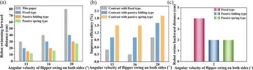
Figure 19(a) shows that with the same swing of the angular velocity of the flippers, the flippers in this paper enable the robot to swim the maximum distance in the water, followed by the fixed type, the passive folding type, and the passive spring type. Moreover, all types of flippers cause the robot to swim forward more quickly as the angular velocity of the flipper increases, but the flipper mechanism proposed in this paper allows the robot to swim forward more quickly than other types of flippers. To obtain the efficiency variability in comparison with other types, the efficiency improvement of the robot based on the flippers of this paper was calculated for the forward swimming distance in the water, as shown in Figure 19(b). From the figure, it is known that as the angular velocity of the swinging flipper increases, the improvement in the efficiency of the flippers in this paper in prompting the robot to swim forward in the water becomes greater than that of other types of flippers. At an angular velocity of 20 rad/s, its efficiency increases by a factor of 1 relative to the fixed type, by a factor of 1.6 relative to the passive folding type, and by a factor of 1.9 relative to the passive spring type. Figure 19(c) is a record of the distance the robot appeared to swim backward within the recovery phase. The fixed type flipper allows the robot to swim backward in the water for a greater distance than the other two types of flippers. Therefore, fixed-type flippers are unable to reduce the angle at which the flipper spreads during the recovery phase. Therefore, the flippers are subjected to a greater water drag force propelled backwards during the retracted swing, which means that the robot can easily swim backward. In contrast, the passive spring and passive folding types can overcome the spring tension or overcome the folding force between opposing surfaces by water drag during the recovery phase, decreasing the angle of their flippers’ opening. This results in less backward-propelled water drag on the flippers during retracted swing. Thus, they are less prone to produce a backwards-swimming robot. However, compared to the flippers proposed in this paper, the passive spring and passive folding types require more water drag to overcome the mechanism of shrinkage and have no active control force, thus producing a poorer effect, and there will be a tendency to swim backward. However, the flippers in this paper can actively control the angle of spreading to narrow during the recovery phase so that the robot, like a frog, can effectively minimize or avoid large water drag during the recovery phase.

6.3. Swimming adaptation performance test in flowing water

To test and verify the effect of the proposed flippers on the swimming performance of the robot in flowing water, a flowing water environment adaptation experiment was carried out, and after processing the experimental video (see Video 3), swimming sequence diagrams of the robot in the water flow subject to the variation factor of the flippers were obtained. Figure 20(i-v) show the swimming sequence diagram of the robot during the propulsion phase in flowing water. As shown in Figure 20 (i), with a flipper spreading angle of 45 degrees at an angular velocity of 15 rad/s, the robot swims forward 17 cm in static water (Va = 0). Compared with Figure 20(ii), when the water flow velocity (V_a) is less than the flipper swing linear velocity (U_M), the robot swims forward the same distance in flowing water as in static water. Thus, the flippers are subjected to very little water drag in the water within the push phase. Compared with Figure 20(iii), when the water flow velocity (V_a) is greater than the flipper swinging linear velocity (U_M), the forward swimming distance of the robot in flowing water is 0. This illustrates that the flippers are subjected to water drag when they swing during the propulsion phase, constraining forward propulsion, which agrees with the hydrodynamic simulation. When the spreading angle of the flippers in Figure 20(iii) was increased to 145 degrees, the robot achieved a forward swimming distance of 20 cm in flowing water, as shown in Figure 20(iv). Moreover, when the flipper swing linear velocity (U_M) in Figure 20(iii) was greater than the velocity Va of the flowing water, the robot achieved forward swimming in the flowing water for a distance of 25 cm. Therefore, when the robot is impacted by the water flow, by increasing the flipper spreading area and swinging angular velocity, the robot is able to overcome the water drag on the flippers and improve the forward propulsive force to make the robot swim forward against the water flow.

Figure 20. Sequence diagram of swimming within the propulsion phase of a robot in flowing water.

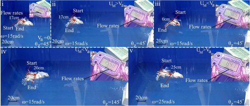
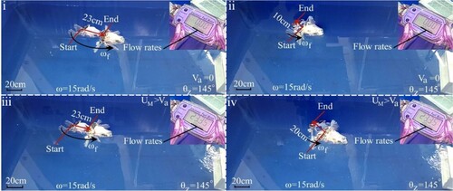
Figure 21(i-iv) show the swimming sequence diagram of the robot during the recovery phase in flowing water. As shown in Figure 21(i), based on the propulsion phase of Figure 20, after a short sliding phase, the spreading angle of the flippers was immediately reduced to a minimum. The flippers were slowly retracted in the opposite direction of ω, the size of which was 2 rad/s, and the robot continued to swim forward for a distance of 23 cm in static water (V_a = 0). Compared to Figure 21(ii), when the flippers were slowly retracted in motion, their spreading angle did not decrease and remained at an angle of 145°, but the robot continued to swim backward for a distance of 10 cm in still water (V_a = 0). Thus, it is illustrated that by reducing the area of the flippers, it is possible to reduce the water drag caused by the flipper retraction movement during the recovery phase, maintaining the forward propulsion of the robot in static water. By applying a certain water flow velocity (V_a) to Figure 21(i), after the flippers immediately change the spreading angle to a minimum and are slowly retracted, the robot is still able to swim forward for a distance of 23 cm in flowing water as shown in Figure 21(iii). Similarly, by applying a certain water flow velocity (V_a) to Figure 21(ii), the impact of the water flow velocity caused the robot to continue to swim backwards for a distance of 20 cm because the spreading angle of the flippers remained at 145 degrees, as shown in Figure 21 (iv). Thus, by reducing the area of the flippers under the impact of water flow, the water drag caused by the retraction of the flipper during the recovery phase can be further reduced, which plays a significant role in maintaining the forward propulsion of the robot in flowing water. In summary, the swimming state realized by the robot in the water flow through the motion characteristics of the flippers in this paper coincides with the regular trend of hydrodynamic simulation and theoretical calculation, thus indirectly verifying that the hydrodynamic simulation and theoretical derivation of the flippers have a certain degree of correctness. Moreover, the frog-like flipper mechanism proposed in this paper not only enables the robot to have good adaptability in a static water environment but also maintains the ability to swim forward against water flow in a water shock environment.

Figure 21. Sequence diagram of swimming within the recovery phase of the robot in flowing water.

7. Conclusion

The flippers are not only the propulsion power device of the frog-like swimming robot, but also the source of bringing water drag. Therefore, its structural form and motion capability have a great influence on the robot's swimming performance in water. At present, the existing flippers cannot be like the frog flippers, which are able to actively adjust the movement change of the flipper area according to the swimming status. To address the above problems, this paper proposes a controllable soft-body extension-driven frog-like flipper mechanism based on the structural form and motion characteristics of frog flippers. It has the characteristics of both rigidity and flexibility and uses a single motor driven by multistage linkage gears, which simulates the frog's precise control of the flipper extension process without the need for additional drive devices, thus making the robot's structure simpler and lighter. By combining the motion equations of the flipper mechanism with the deformation theory of Ogden's super soft-body material, a deformation optimization theoretical model of the flipper was established. Based on the structural parameters of the flipper, with the maximum driving force applied during flipper deformation as the constraint objective, the flipper deformation membrane between the toe bones was optimized. According to the analysis of the force on the frog-like flippers in a simulated water flow field, a fluid dynamics model during paddling was derived. Theoretical calculations and hydrodynamic (CFD) simulations show that flippers are able to instantaneously control the change in the flipper area to inhibit fluid separation during swimming, effectively reducing the water drag of the flippers in flowing water and thus increasing swimming propulsion. Meanwhile, the characteristic curves of the dynamic effects of the flipper spreading angle and swinging angular velocity on swimming propulsion and water drag were also obtained. Finally, the experiment showed that the spreading angle of the flipper not only reached 175 degrees but also that the swimming efficiency was improved by 1, 1.6, and 1.9 times compared with that of the fixed type, passive folding type, and passive spring type flippers, respectively. Moreover, the flippers enable the frog-like swimming robot to reduce water drag, increase propulsive force, and realize good environmental adaptability, as well as high dexterity, in the flowing water environment, thus verifying the feasibility and rationality of the design structure.

Compared to the other three types of flipper mechanisms in this paper, this frog-like flipper mechanism allows the robot to achieve improved results in terms of the swimming performance in water, but there are still some limitations. The characteristic mechanism of frog flippers involves many factors, such as the toe joints being bent and the flippers undergoing multi-dimensional rotation. The main aim of this paper is to study and analyse the hydrodynamic motion that can change the contact area with water and the angular velocity of frog flippers while swimming, with a focus on the feasibility of simplifying the design of the frog flipper mechanism. In the experiments, due to the limitations of time and cost, it is difficult to obtain the required propulsive force and water resistance directly when the experimental prototype is swimming in a water environment. Thus, we obtain data on the swimming distance and turning angle, which can be used to indirectly verify the feasibility and reasonableness of the relevant simulation analysis, the theoretical derivation, and the design structure. In the follow-up research, we will consider more frog flipper characteristic mechanism factors and further optimize the design of the flipper structure. Meanwhile, more design parameters and experimental methods will be used to directly verify the theoretical analysis problems of the relevant structural models. So as to further explore the potential of the frog-like flipper mechanism enables the frog-like swimming robot to obtain the power rapid response in swimming, and ultimately to achieve the power effect of real frog flippers. In addition, based on the theoretical model of the frog-like flipper mechanism constructed in this paper, combined with improvements in frog-like jumping and swimming mechanisms, this mechanism can be applied to the research and development of frog-like amphibious robot technology and practical engineering applications in the future.

Disclosure statement

No potential conflict of interest was reported by the author(s).

Additional information

Funding

The authors gratefully acknowledge support from National Key Research and Development Plan “intelligent robot” key project (2019YEB1309600),the National Key Research and Development Program of China ‘Intelligent Robot’ key special project (2017YFB1300104), National Natural Science Foundation of China (51675124) ‘Research on the mechanism of frog-inspired amphibious robot musculoskeletal system for complex environment applications’, State Key Laboratory of Robotics and System (Harbin Institute of Technology) independent research ‘Research on Key Technology of Frog-inspired Soft Robot Based on Explosion Drive’ (SKLRS201703A), National Natural Science Foundation of China (U2013214), and Self-Planned Task of State Key Laboratory of Robotics and System (HIT) (SKLRS202001A03).

Appendix

Appendix 1

In Figure 6(c), the line segments JJ₁ and HH₁ are the initial positions of the toe bone (e and f), respectively. When toe bone e is rotated by (θ₃) at angular velocity (W_e), the position is line segment O₄J₂. At the same time, toe bone f rotates (θ₄) with angular velocity (W_f), and its position is line segment O₅H₃. At this point, the area of deformation of the soft-body membrane movement between the toe bones (c, e and f) is shown as sector J₁J₂H₃O₅FF₁ in the figure. Because the length difference between the toe bones is not large, points F₁J₁ are linked by a straight line, points J₁J₂ are connected by an arc with point O₄ as the centre of the circle, and points J₂H₃ are connected by a straight line. Therefore, the area of sector J₁J₂H₃O₅FF₁ is similar to that of the polygon J₁J₂H₃O₅FF₁.

To derive the mapping relationship between the motion joint angle of the right toe bone and the motion area of the flipper, the deformed area of polygon J₁J₂H₃O₅FF₁ is divided into S5, S6, S7, S8, and ΔJO₅O₄. Here, the areas of S5 and ΔJO₅O₄ are determined by the dimensions of the structure, which are fixed values, and the values are so small that they can be ignored. Thus, the motion area of the right flipper can be obtained as the S_Y: (1-1) $\begin{array}{r}{S}_Y=S_{S6}+S_{S7}+S_{S8}\end{array}$(1-1) The movement area of S5 is generated by the movement of toe bone (e) by rotating (θ₃) in the centre of circle O₄, so the movement area of S6 is expressed as follows: (2-2) $\begin{array}{r}{S}_{S6}=\frac{{\theta }_3\pi }{{360}^{\circ }}\bullet (O_4{J}_1{)}^2\end{array}$(2-2) Similarly, the movement areas of S7 and S8 are generated by the movement of toe bone f relative to toe bone e, so the extension line is formed along the direction FO₅, intersecting the vertically downward extension line of point H₃ and perpendicular to point I₁. Furthermore, a vertical line is generated from point O₄ to line segment H₃I₁ with respect to point I. The angle of ∠H₁O₅H₃ is known to be θ₄, so the angle of ∠H₃O₅I₁ is 90°- θ₄, and the line segment H₃O₅ is the length of toe bone f. Therefore, the expressions for the lengths of lines H₃I₁ and I₁O₅ are as follows: (3-3) $\begin{array}{r}\{\begin{array}{l}{L}_{H_3{I}_1}=\sin \left({\displaystyle \frac{\pi }{2}}-{\theta }_4\right)\ast H_3{O}_5\\ L_{I_1{O}_5}=\cos \left({\displaystyle \frac{\pi }{2}}-{\theta }_4\right)\ast H_3{O}_5\end{array}\end{array}$(3-3) It is known that the quadrangle JO₄H₃I₁ is a right-angle trapezoid, the upper side O₄J = JO₅= L₁, and the height is $L_{I_1{O}_5}+L_1$; thus, the trapezoid change area S_TT is expressed as follows: (4-4) $\begin{array}{r}{S}_{\mathrm{TT}}=\frac{\left(L_{H_3{I}_1}+L_1\right)\ast \left(L_{I_1{O}_5}+L_1\right)}{2}\end{array}$(4-4) Similarly, ΔH₃O₅I₁ is a right triangle, and the area of change in the triangle can be obtained by formula (3-3), whose expression is as follows: (5-5) $\begin{array}{r}{S}_{\mathrm{\Delta }{H}_3{O}_5{I}_1}=(H_3{O}_5{)}^2\ast \sin \left(2\ast \left(\frac{\pi }{2}-{\theta }_4\right)\right)/4\end{array}$(5-5) The area of the trapezoid S_TT is composed of ΔO₅O₄J, ΔO₅I₁H₃ and S8, of which ΔO₅O₄J is very small and negligible. The expression for the area of motion of S8 can be obtained from formulas (4-4) and (5-5): (6-6) $\begin{array}{r}{S}_{S8}=\frac{\begin{array}{c}2\ast \left(L_{H_3{I}_1}+L_1\right)\ast \left(L_{I_1{O}_5}+L_1\right)\\ -{\left(H_3{O}_5\right)}^2\ast \sin \left(2\ast \left(\frac{\pi }{2}-{\theta }_4\right)\right)\end{array}}{4}\end{array}$(6-6) To easily calculate the area S7 of ΔO₄H₃J₂, high lines are made from point H₃ to side J₂O₄, intersecting at point H₂. Given that the angle of ∠J₁O₄I is 90 degrees, the angle change expression of ∠J₂O₄H₃ is obtained as follows: (7-7) $\begin{array}{r}\mathrm{\angle }{J}_2{O}_4{H}_3=\frac{\pi }{2}-\left({\theta }_3+\mathrm{\angle }{H}_3{O}_{4}I\right)\end{array}$(7-7) According to the lengths of sides H₃I and IO₄ in the right triangle ΔH₃O₄I, the expression for the change in the angle ∠H₃O₄I and the length of the H₃O₄ line segment can be found as follows: (8-8) $\begin{array}{r}\{\begin{array}{l}\mathrm{\angle }{H}_3{O}_{4}I=\arctan \left(\frac{L_{H_3{I}_1}-L_1}{L_{I_1{O}_5}+L_1}\right)\\ L_{H_3{O}_4}=\sqrt{{\left(L_{H_3{I}_1}-L_1\right)}^2+{\left(L_{I_1{O}_5}+L_1\right)}^2}\end{array}\end{array}$(8-8) From formula (8-8) and (7-7), the high line H₃H₂= sin (∠J₂O₄H₃) * H₃O₄ in ΔO₄H₃J₂, and the area expression of S7 can be calculated based on the triangle area formula: (9-9) $\begin{array}{rl}{S}_{S7}& =(\sqrt{{\left(L_{E_{2}E}-L_1\right)}^2+{\left(L_{E{O}_3}+L_1\right)}^2}\\ & \ast \sin \left(\mathrm{\angle }{J}_2{O}_4{H}_3\right)\ast J_2{O}_4)/2\end{array}$(9-9)

Appendix 2

Figure A1. Tensile experimental test of the soft membrane material of the sub-flippers.

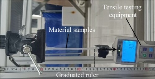
As shown in figure A1, samples with an initial width (ΔR) of 10 mm, initial length (ΔL) of 20 mm, and initial thickness (ΔK) of 0.5 mm, 1 mm, 1.5 mm, 2 mm, 2.5 mm, and 3 mm were taken first. The above samples with different initial thicknesses (ΔK) were tensioned under a certain tensile force (F), and the elongation limit value (ΔLL) and the corresponding tensile force (F) value of the test samples were then tested. The experimental data are shown in Table A1.

Table A1. Data value.

Initial thicknesses (ΔK) (mm)	Elongation limit value (ΔLL) (mm)	Tensile force F (N)
0.5	80	1.7
1	100	4.4
1.5	120	11.7
2	130	18.1
2.5	150	22.8
3	160	31.3

At the same time, samples with an initial width (ΔR) of 10 mm, initial thickness value ΔK of 1 mm, and initial length (ΔL) of 5 mm, 10 mm, 15 mm, 20 mm, 25 mm, and 30 mm, respectively, were then selected. The above samples with different initial length (ΔL) were tensioned under a certain tensile force (F), and the elongation limit value (ΔLL) and the corresponding tensile force (F) value of the test samples were tested. The experimental data are shown in Table A2.

Table A2. Data value.

Initial length (ΔL) (mm)	Elongation limit value (ΔLL) (mm)	Tensile force F (N)
5	40	3.1
10	65	3.9
15	80	4.5
20	100	5.2
25	140	6.6
30	180	7.9

Appendix 3

As shown in Figure 7, where the width of the sub-flipper is approximated by the length (R_i) of the toe bone (i), the expression is as follows: (A-1) $\begin{array}{r}\{\begin{array}{l}{R}_1\approx R_a=65\mathrm{mm}\\ R_2\approx R_b=70\mathrm{mm}\\ R_3\approx R_e=85\mathrm{mm}\\ R_4\approx R_f=77\mathrm{mm}\end{array}\end{array}$(A-1) Where R₁, R₂, R₃, and R₄ denote the width of sub-flippers 1, 2, 3, and 4. From the above conclusions, it can be seen that under certain limit conditions, the initial thickness is chosen to be smaller, and the initial length is chosen to be longer so that larger elongation values can be realized under a relatively small tensile force. Therefore, to maintain a certain degree of elasticity in the sub-flipper material, the sub-flipper touch thickness values K are all taken as 1 mm. It is assumed that the limiting angle of the servo input in the frog-like flipper mechanism is [0°, 90°], and under this angular range of inputs, the flipper mechanism is only subjected to the tensile force of the sub-flippers and is optimized with the servo output torque (T:14 kg.cm) as the target. With the known RPM ratio between the toe bones (i) and the servo, the approximate torque acting on each toe bone can be found as follows: (A-2) $\begin{array}{r}\{\begin{array}{l}{T}_1=2.7\mathrm{kg}\cdot \mathrm{cm}\\ T_2=4.2\mathrm{kg}\cdot \mathrm{cm}\\ T_3=-4.2\mathrm{kg}\cdot \mathrm{cm}\\ T_4=-2.7\mathrm{kg}\cdot \mathrm{cm}\end{array}\end{array}$(A-2) Where T₁, T₂, T₃, and T₄ are the torques acting on the toe bones (i) in the sub-flippers. Since torque = force arm * force at the end, based on Equation (A-1), the tension force F_i is determined at the end of each toe bone, with the following values: (A-3) $\begin{array}{r}\{\begin{array}{l}{F}_a=4.15N\\ F_b=6N\\ F_e=-6N\\ F_f=-4.15N\end{array}\end{array}$(A-3) As the length of the toe bone (i) becomes increasingly shorter and closer to the centre of rotation, the tension force on it increases. To facilitate the calculation and solution in the optimization, it is assumed that the force acting on the toe bone (i) is uniform, and the value is the toe bone end force F_i, which has a uniform width unit of 1 mm. Therefore, by setting the value of the research unit ΔR_i in Equation (19) to 1 mm, M_i on the toe bone in the sub-flippers can be obtained. its value is as follows: (A-4) $\begin{array}{r}\{\begin{array}{l}{M}_a=65\\ M_b=70\\ M_e=85\\ M_f=77\end{array}\end{array}$(A-4) From the relative movement distance between the ends of the toe bone (i) in figure 10(c), the elongation (ΔL_i,1) value of the elongation of the tensile end of the sub-flippers can be obtained. However, the distance of movement between the ends of the toe bones (i) also decreases as the length of the toe bones decreases. The distance of movement between the ends of the phalanges is small when the toe bone length is 0, at which point the elongation of the sub-flippers is always close to zero. Therefore, the elongation (ΔL_i,1) has the following range of values: (A-5) $\begin{array}{r}\{\begin{array}{l}0<\mathrm{\Delta }{L}_{a,1}\le 36\mathrm{mm}\\ 0<\mathrm{\Delta }{L}_{b,1}\le 46.2\mathrm{mm}\\ 0<\mathrm{\Delta }{L}_{e,1}\le 85\mathrm{mm}\\ 0<\mathrm{\Delta }{L}_{f,1}\le 75\mathrm{mm}\end{array}\end{array}$(A-5)

Appendix 4

Figure A2. Hydrodynamic simulation analysis based on the spreading angle of the flippers: (a) mesh delineation of the flipper model; (b) flipper spreading angle (θ_Z) of 20°; (c) flipper spreading angle (θ_Z) of 60°; (d) flipper spreading angle (θ_Z) of 100°; (e) flipper spreading angle (θ_Z) of 140°; and (f) flipper spreading angle (θ_Z) of 180°.

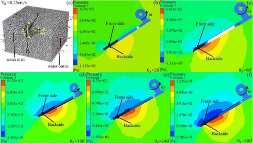
We randomly obtained two symmetrical points on the front and back surfaces of the flippers (point F for the front side and point B for the back side), recorded the data of the changes in these two points, and plotted the data in Figure 15(b,c). Because the flipper surface changes nearly uniformly, at any position on the two symmetric flipper points in the simulation calculation, the general trend of the change in the data is the same. The description is as follows:

Figures A2(b-f) show the flipper under a certain water flow velocity and flipper swing angle velocity. The flipper spreading angle is modified to change the area of mutual contact with the water and the pressure cloud of the simulation calculation in the fluent module. The settings of the k-ϵ turbulence model are as follows: the inlet water flow velocity (V_a) is 0.25 cm/s, the angular velocity (ω) of the flipper swing is 10 rad/s, and the angles (θ_Z) of flipper spreading are 20°, 60°, 100°, 140° and 180°. The left-hand legend in the pressure cloud figure shows the scale values of the pressure change, the magnitude of which gradually increases from bottom to top as the colour changes. Conversely, it decreases.

As the flipper spreading angle increases, the layers of the colour region of the pressure cloud map on the back of the flipper in figures A2(b-f) become increasingly numerous, and the colour gradually changes to red toward the flipper surface. Moreover, the area of the same-coloured region also increases gradually with an increasing angle of flipper spreading. Therefore, the corresponding legend values increase. The point B simulation data are approximately 450.12 Pa, 536.23 Pa, 642.15 Pa, 769.02 Pa, and 880.12 Pa, respectively. Similarly, as the angle of flipper spreading increases, the layers of the colour region of the pressure cloud map on the front side of the flipper in figures A2(b-f) become increasingly numerous, and the colour gradually changes to darker blue towards the flipper surface. Moreover, the area of the same-coloured region also gradually increases with an increasing angle of flipper spreading. As a result, the corresponding legend values are decreasing. The point F simulation data are approximately 308.56 Pa, 217.33 Pa, 120.65 Pa, 60.12 Pa, and −10.13 Pa, respectively.

Figure A3. Hydrodynamic simulation analysis of the flippers under a change in inlet water flow velocity: (a) water velocity (V_a) of 0.1 cm/s; (b) water velocity (V_a) of 0.3 cm/s; (c) water velocity (V_a) of 0.6 m/s; (d) water velocity (V_a) of 0.9 cm/s; (e) water velocity (V_a) of 1.2 cm/s; and (f) water velocity (V_a) of 1.4 cm/s.

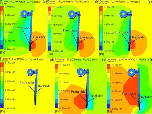
Figures A3 (a-f) show the flipper under a certain flipper swing linear velocity and flipper spreading angle. By changing the inlet water flow velocity to change the impact force on the flipper, the pressure cloud of the simulation calculation in the fluent module changes. By setting the k-ϵ turbulence model, the linear velocity (U_m) of the flipper swing is 0.9 cm/s, and the flipper spreading angle (θ_Z) is 100°. The inlet water velocities (V_a) are 0.1, 0.3, 0.6, 0.9, 1.2, and 1.4 cm/s. The left-hand legend in the pressure cloud figure shows the scale values of the pressure change, the magnitude of which gradually increases from bottom to top as the colour changes. Conversely, it decreases. The following three cases are considered:

When the linear velocity of the flipper swing is greater than the inlet water flow velocity, as the inlet water flow velocity increases, the layers of the colour regions of the pressure maps on the back of the flippers in figures A3 (a-c) have the same number of layers, and the colours and the areas of the same colour regions are all the same. Therefore, the corresponding legend values are approximately the same. The point B simulation data are approximately 710.12, 711.01, and 710.23 Pa, respectively. Similarly, as the velocity of the inlet water flow increases, the layers of the colour area of the pressure cloud map on the front side of the flippers in figures A3(a-c) become increasingly fewer, but the colours gradually become lighter yellow towards the flipper surface, and the area of the same colour region gradually becomes increasingly larger. Therefore, the corresponding legend values increase. The point F simulation data are approximately 210.11, 254.24, and 310.13 Pa, respectively.

When the linear velocity of the flipper swing is equal to the velocity of the inlet water flow, the pressure cloud maps on the front and the back of the flipper in figure A3(d) show the same colours, with the colour areas in the same layer. Therefore, the corresponding legend values are approximately the same. The simulation data at points F and B are approximately 711.13 and 711.06 Pa, respectively.

When the linear velocity of the flipper swing is smaller than the inlet water flow velocity, as the inlet water flow velocity increases, the layers of the colour region of the pressure cloud maps on the back of the flippers in figures A3(e-f) become increasingly numerous, the colour gradually becomes lighter blue towards the flipper face, and the area of the same colour region becomes increasingly larger. As a result, the corresponding legend values decrease. The point B simulation data are approximately 413.63 and 352.24 Pa, respectively. Similarly, as the velocity of the inlet water flow increases, the layers and colours of the colour regions of the pressure cloud maps on the front of the flippers in figure A3(e-f) remain almost unchanged and gradually become reddish towards the flipper face, and the area of the same region of colour increases. Therefore, the corresponding legend values increase. The point F simulation data are approximately 1106.12 and 1310.07 Pa, respectively.

Appendix 5

Figure A4. Swimming sequence diagram of the robot with the flippers spread at an angle (θ_z) of 85°: (a) motion of the robot's flippers during three stages in water; (b) angular velocity (ω) of the flippers swinging on both the right and left sides of 20 rad/s; (c) angular velocity (ω) of the flippers swinging on both the right and left sides of 16 rad/s; angular velocity (ω) of the flippers swinging on both the right and left sides of 13 rad/s. (L_y in figures (b-d) represents the distance the robot swam forward.)

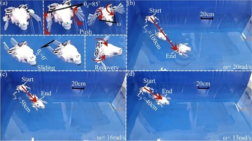
Figure A5. Swimming sequence diagram of the robot with the flippers spread at an angle (θ_z) of 155°: (a) motion of the robot's flippers during three stages in water; (b) angular velocity (ω) of the flippers swinging on both the right and left sides of 20 rad/s; (c) angular velocity (ω) of the flippers swinging on both the right and left sides of 16 rad/s; angular velocity (ω) of the flippers swinging on both the right and left sides of 13 rad/s. (Ly in figures (b-d) represents the distance the robot swam forward.)

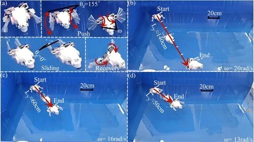
Figure A6. Sequence diagram of the robot turning swimming: (a) motion state of the robot's flippers during three stages in water; (b) flipper spreading angles (θ_z1 and θ_z2) were respectively 20 and 155 rad/s; (c) flipper spreading angles (θ_z1 and θ_z2) were respectively 20 and 85 rad/s; (d) flipper spreading angles (θ_z1 and θ_z2) were respectively 20 and 65 rad/s. (θ_z1 denotes the flipper spreading angle of the left side, and θ_z2 denotes the flipper spreading angle of the right side;)

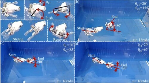
Appendix 6

Figure A7. Experimental tests of swimming in water for a robot based on fixed-type flippers: (a) angular velocity (ω) of the swinging flipper is 20 rad/s for both sides; (b) angular velocity (ω) of the swinging flipper is 16 rad/s for both sides; (c) angular velocity (ω) of the swinging flipper is 13 rad/s for both sides; and (d) backward swimming test is generated during the recovery phase. (L_y in figures (a-c) represents the distance the robot swam forward; and L_y in figure (d) represents the distance the robot swims backward.)

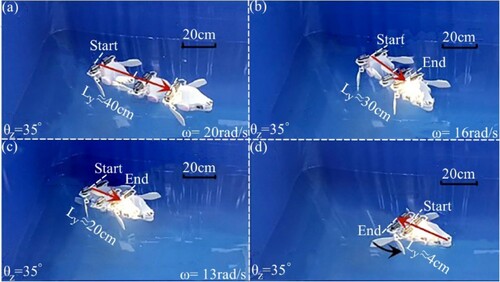
Figure A8. Experimental tests of swimming in water for a robot based on passive folding type flippers: (a) angular velocity (ω) of flipper swinging is 20 rad/s for both sides; (b) angular velocity (ω) of flipper swinging is 16 rad/s for both sides; (c) angular velocity (ω) of flipper swinging is 13 rad/s for both sides; and (d) backward swimming test is generated during the recovery phase. (L_y in figure (a-c) represents the distance the robot swam forward; L_y in Figures (d) represents the distance the robot swims backwards).

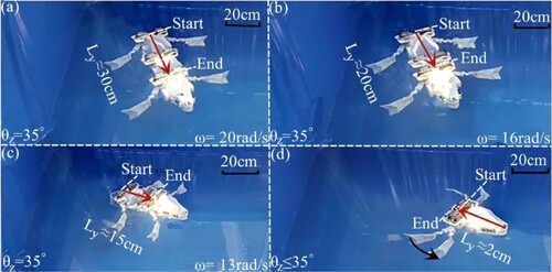
Figure A9. Experimental tests of swimming in water for a robot based on passive spring type flippers: (a) angular velocity (ω) of flipper swinging is 20 rad/s for both sides; (b) angular velocity (ω) of flipper swinging is 16 rad/s for both sides; (c) angular velocity (ω) of flipper swinging is 13 rad/s for both sides; and (d) backward swimming test is generated during the recovery phase. (L_y in figure (a-c) represents the distance the robot swam forward; L_y in Figures (d) represents the distance the robot swims backwards).

References

- Abdelsalam, S. I., Abbas, W., Megahed, A. M., & Said, A. A. M. (2023). A comparative study on the rheological properties of upper convected Maxwell fluid along a permeable stretched sheet. Heliyon, 9(12), e22740. https://doi.org/10.1016/j.heliyon.2023.e22740
- Baines, R., Fish, F., & Kramer-Bottiglio R. (2021). Amphibious robotic propulsive mechanisms: Current technologies and open challenges. Bioinspired Sensing, Actuation, and Control in Underwater Soft Robotic Systems, 2021, 41–69. https://doi.org/10.1007/978-3-030-50476-2_3
- Baines, R., Patiballa, S. K., Booth, J., Ramirez, L., Sipple, T., Garcia, A., Fish, F., & Kramer-Bottiglio, R. (2022). Multi-environment robotic transitions through adaptive morphogenesis. Nature, 610(7931), 283–289. https://doi.org/10.1038/s41586-022-05188-w
- Bhatti, M. M., Vafai, K., & Abdelsalam, A. I. (2023). The role of nanofluids in renewable energy engineering. Nanomaterials, 13(19), 2671. https://doi.org/10.3390/nano13192671
- Cai, W., Tao, C., Wang, Y., Wu, T., Xu, C., & Zhang, G. (2023). Applications of autonomous underwater vehicle in submarine hydrothermal fields: A review. Robot, 45(4), 483–495.
- Chen, G., Tu, J., Ti, X., Wang, Z., & Hu, H. (2021). Hydrodynamic model of the beaver-like bendable webbed foot and paddling characteristics under different flow velocities. Ocean Engineering, 234, 109179. https://doi.org/10.1016/j.oceaneng.2021.109179
- Dong, H., Wu, Z., Chen, D., Tan, M., & Yu, J. (2020). Development of a whale-shark-inspired gliding robotic fish with high maneuverability. IEEE/ASME Transactions on Mechatronics, 25(6), 2824–2834. https://doi.org/10.1109/TMECH.2020.2994451
- Esposito, C. J., Tangorra, J. L., Flammang, B. E., & Lauder, G. V. (2012). A robotic fish caudal fin: Effects of stiffness and motor program on locomotor performance. Journal of Experimental Biology, 215(1), 56–67. https://doi.org/10.1242/jeb.062711
- Fan, J., Du, Q., Dong, Z., Zhao, J., & Xu, T. (2022). Design of the Jump mechanism for a biomimetic robotic frog. Biomimetics, 7(4), 142. https://doi.org/10.3390/biomimetics7040142
- Fu, S., Wei, F., Yin, C., Yin, C., Yao, L., & Wang, Y. (2021). Biomimetic soft micro-swimmers: From actuation mechanisms to applications. Biomedical microdevices, 23(1), 6. https://doi.org/10.1007/s10544-021-00546-3
- Gul, J. Z., Kim, K. H., Lim, J. H., Doh, Y. H., & Choi, K. H. (2017). FSI modeling of frog inspired soft robot embedded with ALD encapsulated flex sensor for underwater synchronous swim. In: IEEE International Symposium on Robotics and Intelligent Sensors (IRIS), IEEE, pp. 255–259.
- Kabanov, A., Kramar, V., & Ermakov, I. (2021). Design and modeling of an experimental ROV with six degrees of freedom. Drones, 5(4), 113. https://doi.org/10.3390/drones5040113
- Keithly, D., Whitehead, J., Voinea, A., Horna, D., Hollenberg, S., Peck, M., Pikul, J., Robert, F., & Shepherd, R. F. (2018). A cephalopod-inspired combustion powered hydro-jet engine using soft actuators. Extreme Mechanics Letters, 20, 1–8. https://doi.org/10.1016/j.eml.2017.11.007
- Ko, J., Kim, C., Lim, D., Song, Y., Lee, S., Yeom, B., Huh, J., Han, S., Kang, D., Koh, J., & Cho, J. (2022). High-performance electrified hydrogel actuators based on wrinkled nanomembrane electrodes for untethered insect-scale soft aquabots. Science Robotics, 7(7), eabo6463. https://doi.org/10.1126/scirobotics.abo6463
- Li, Q., Chen, T., Chen, Y., & Wang, Z. (2023). An underwater bionic crab soft robot with multidirectional controllable motion ability. Ocean Engineering, 278, 114412. https://doi.org/10.1016/j.oceaneng.2023.114412
- Lin, D., Yang, F., Gong, D., & Li, R. (2023). Bio-inspired magnetic-driven folded diaphragm for biomimetic robot. Nature Communications, 14(1), 163. https://doi.org/10.1038/s41467-023-35905-6
- Liu, J., Yu, F., He, B., & Yan, T. (2022a). Hydrodynamic numerical simulation and prediction of bionic fish based on computational fluid dynamics and multilayer perceptron. Engineering Applications of Computational Fluid Mechanics, 16(1), 858–878. https://doi.org/10.1080/19942060.2022.2052355
- Liu, Y., Li, H., Deng, S., Wang, S., Liu, S., & Wang, Z. (2022b). Biomimetic robotic sea lion Foreflippers: Design, modeling, and experimentation. IEEE/ASME Transactions on Mechatronics, 27(6), 5679–5689. https://doi.org/10.1109/TMECH.2022.3187014
- Lu, C., Sun, J., & Qi, S. (2016). Dynamics and simulation analysis of the bionic frog robot in takeoff phase. Applied Science and Technology, 43(1), 51–55 + 80.
- Nwafor, C. J., Girerd, C., Laurent, G. J., Morimoto, T. K., & Rabenorosoa, K. (2023). Design and fabrication of concentric tube robots: A Survey. IEEE Transactions on Robotics, 39(4), 2510–2528. https://doi.org/10.1109/TRO.2023.3255512
- Pan, Y., Fan, J., Liu, G., Liu, Y., & Zhao, J. (2024). Design and kinematic analysis of a rope-driven linkage frog-like swimming robot with multidirectional controllable motion. Ocean Engineering, 291, 1–15.
- Pan, Y., Fan, J., Ma, W., Gao, F., Liu, G., & Zhao, J. (2023). Design and motion analysis of a frog-like jumping robot based on a soft body detonation drive. Materials & Design, 232, 1–15.
- Shen, Y., Harada, N., Katagiri, S., & Tanaka, H. (2021). Biomimetic realization of a Robotic Penguin Wing: Design and thrust characteristics. IEEE/ASME Transactions on Mechatronics, 26(5), 2350–2361. https://doi.org/10.1109/TMECH.2020.3038224
- Shimizu, M., Ishii, D., Aonuma, H., & Hosoda, K. (2017). Swimming frog cyborg which generates efficient hydrodynamic propulsion with webbed foot. IEEE International Conference on Cyborg and Bionic Systems (CBS), Beijing, China, pp. 73–76.
- Shin, J., Jamil, B., Moon, H., Koo, J. C., Choi, H. R., & Rodrigue, H. (2022). Thermo-pneumatic artificial muscle: Air-based thermo-pneumatic artificial muscles for pumpless pneumatic actuation. Soft Robotics, 11(2), 187–370.
- Su, X., Pan, Q., Wang, H., & Ren, Z. (2021). Research progresses of robots with active deformable materials. Robot, 43(1), 112–128.
- Sun, T., Chen, G., Yang, S., Wang, Y., Wang, Y., Tan, H., & Zhang, L. (2021). Design and optimization of a bio-inspired hull shape for AUV by surrogate model technology. Engineering Applications of Computational Fluid Mechanics, 15(1), 1057–1074. https://doi.org/10.1080/19942060.2021.1940287
- Wang, S., Fan, J., Pan, Y., Liu, G., & Liu, Y. (2024). Design and analysis of adaptive flipper with origami structure for frog-inspired swimming robot. IEEE Robotics and Automation Letters, 9(2), 1262–1269. https://doi.org/10.1109/LRA.2023.3333674
- Wang, Y., Deng, J., Li, T., Liu, K., Liu, H., & Ma, S. (2021). Review of research on 3D printing manufacturing technology of soft robots. Journal of Mechanical Engineering, 57(15), 186–198. https://doi.org/10.3901/JME.2021.15.186
- Wei, W., Tao, T., Si, L., Wang, G., & Yan, Q. (2023). Design and optimization of bionic Nautilus volute for a hydrodynamic retarder. Engineering Applications of Computational Fluid Mechanics, 17(1), 2273391. https://doi.org/10.1080/19942060.2023.2273391
- Xia, P., You, H., Ye, Y., & Du, J. (2023). ROV teleoperation via human body motion mapping: Design and experiment. Computers in Industry, 150, 103959. https://doi.org/10.1016/j.compind.2023.103959
- Yan, Z., Yang, H., Zhang, W., Lin, F., Gong, Q., & Zhang, Y. (2022). Bionic fish tail design and trajectory tracking control. Ocean Engineering, 257, 111659. https://doi.org/10.1016/j.oceaneng.2022.111659
- Zhang, K., Zhang, S., Chen, H., & Yu, C. (2023a). Research on underwater gait generation of the amphibious. Mechanical Science and Technology for Aerospace Engineering, 1–6.
- Zhang, Y., Kong, D., Shi, Y., Cai, M., Yu, Q., Li, S., Wang, K., & Liu, C. (2023b). Recent progress on underwater soft robots: Adhesion, grabbing, actuating, and sensing. Frontiers in Bioengineering and Biotechnology, 11, 1196922. https://doi.org/10.3389/fbioe.2023.1196922
- Zhao, W., Zhang, Y., Lim, K. L., Luo, J., & Wang, N. (2022). Development and performance analysis of pneumatic soft-bodied bionic flipper. Advanced Engineering Materials, 24(8), 2101566. https://doi.org/10.1002/adem.202101566
- Zhu, Q., & Bi, X. (2017). Effects of stiffness distribution and spanwise deformation on the dynamics of a ray-supported caudal fin. Bioinspiration & Biomimetics, 12(2), 026011. https://doi.org/10.1088/1748-3190/aa5d3f
Appendix
Appendix 1
In Figure (c), the line segments JJ1 and HH1 are the initial positions of the toe bone (e and f), respectively. When toe bone e is rotated by (θ3) at angular velocity (We), the position is line segment O4J2. At the same time, toe bone f rotates (θ4) with angular velocity (Wf), and its position is line segment O5H3. At this point, the area of deformation of the soft-body membrane movement between the toe bones (c, e and f) is shown as sector J1J2H3O5FF1 in the figure. Because the length difference between the toe bones is not large, points F1J1 are linked by a straight line, points J1J2 are connected by an arc with point O4 as the centre of the circle, and points J2H3 are connected by a straight line. Therefore, the area of sector J1J2H3O5FF1 is similar to that of the polygon J1J2H3O5FF1.